Bayesian robust correlation with Stan in R
(and why you should use Bayesian methods)
Adrian Baez-Ortega
28 May 2018
While looking for a Bayesian replacement for my in-house robust correlation method (Spearman’s correlation with bootstrap resampling), I found two very interesting posts on standard and robust Bayesian correlation models in Rasmus Bååth’s blog. As I wanted to give the robust model a try on my own data (and also combine it with a robust regression model) I have translated Bååth’s JAGS code into Stan and wrapped it inside a function. Below I show how this model is more suitable than classical correlation coefficients, regardless of whether the data are normally distributed.
As Rasmus Bååth explains in his first blog post on Bayesian correlation:
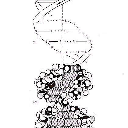
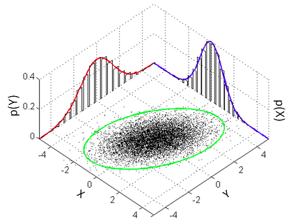
The model that a classical Pearson’s correlation test assumes is that the data follows a bivariate normal distribution. That is, if we have a list x of pairs of data points [[x1,1, x1,2], [x2,1, x2,2], [x3,1, x3,2], …] then the xi,1s and the xi,2s are each assumed to be normally distributed with a possible linear dependency between them. This dependency is quantified by the correlation parameter ρ which is what we want to estimate in a correlation analysis. A good visualization of a bivariate normal distribution with ρ = 0.3 can be found on the the wikipedia page on the multivariate normal distribution :
The bivariate normal model described later in the same post is equivalent to the classical Pearson’s correlation coefficient, and it suffers from the same problems. Because Pearson’s correlation assumes that the data come from a bivariate normal distribution (i.e. that the observations for each of the two variables are normally distributed), it is very sensitive to outliers. Since a truly normal distribution cannot accommodate serious outliers, the normal distributions are skewed towards them, which results in a reduction in the estimated correlation coefficient. The usual way to address this when using non-normal data in classical statistics is through Spearman’s rank correlation coefficient, which is more robust to outliers. However, Spearman’s is not simply a robust version of Pearson’s coefficient, but they actually measure different things: while Pearson’s correlation measures the strength of a linear relationship between the two variables, Spearman’s correlation measures the strength of a monotonic relationship between the variables. So there is no truly robust version of Pearson’s correlation coefficient available in traditional statistics.
In Bayesian statistics, however, the correlation model can be made robust to outliers quite easily, by replacing the bivariate normal distribution by a bivariate Student’s t-distribution, as Bååth explains in his second post on Bayesian correlation:
What you actually often want to assume is that the bulk of the data is normally distributed while still allowing for the occasional outlier. One of the great benefits of Bayesian statistics is that it is easy to assume any parametric distribution for the data and a good distribution when we want robustness is the t-distribution. This distribution is similar to the normal distribution except that it has an extra parameter ν (also called the degrees of freedom) that governs how heavy the tails of the distribution are. The smaller ν is, the heavier the tails are and the less the estimated mean and standard deviation of the distribution are influenced by outliers. When ν is large (say ν > 30) the t-distribution is very similar to the normal distribution. So in order to make our Bayesian correlation analysis more robust we’ll replace the multivariate normal distribution from the last post with a multivariate t-distribution. To that we’ll add a prior on the ν parameter
nuthat both allows for completely normally distributed data or normally distributed data with an occasional outlier.
Adopting a multivariate t-distribution with a vague prior on its degrees of freedom makes Bååth’s robust model inherently adaptable to the level of noise. That is, if the data are strictly normal, nu will be estimated to be very large, and the model will be equivalent to the one with a bivariate normal distribution; but if the data are noisy, then nu will be estimated to an appropriately small value, and the resulting multivariate t-distribution will inherently incorporate the outliers in the data without this having an effect on the correlation coefficient. This is very nicely shown in Bååth’s post, but I will illustrate it below using the Stan version of his model.
Let’s try the model on some artificial correlated data in R. We will need the following packages:
library(rstan)    # to run the Bayesian model (stan)
library(coda)     # to obtain HPD intervals (HPDinterval)
library(mvtnorm)  # to generate random correlated data (rmvnorm)
library(car)      # to plot the inferred distribution (dataEllipse)
We can generate random data from a multivariate normal distribution with pre-specified correlation (rho) using the rmvnorm function in the mvtnorm package. The covariance matrix is constructed as explained in Rasmus Bååth’s post.
sigma = c(20, 40)
rho = -0.95
cov.mat = matrix(c(sigma[1] ^ 2,
                   sigma[1] * sigma[2] * rho,
                   sigma[1] * sigma[2] * rho,
                   sigma[2] ^ 2),
                 nrow=2, byrow=T)

set.seed(210191)
x.clean = rmvnorm(n=40, sigma=cov.mat)
plot(x.clean, pch=16)
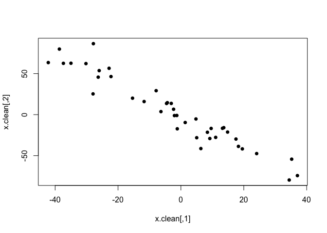
Let’s first take a look at the classical correlation coefficients (Pearson’s and Spearman’s) on these data.
cor(x.clean, method="pearson")[1, 2]
## [1] -0.959702
cor(x.clean, method="spearman")[1, 2]
## [1] -0.9581614
These data are a bit too clean for my taste, so let’s introduce some extreme outliers.
x.noisy = x.clean
x.noisy[1:3,] = matrix(c(-40, -60,
                         20, 100,
                         40, 40),
                       nrow=3, byrow=T)
plot(x.noisy, pch=16)
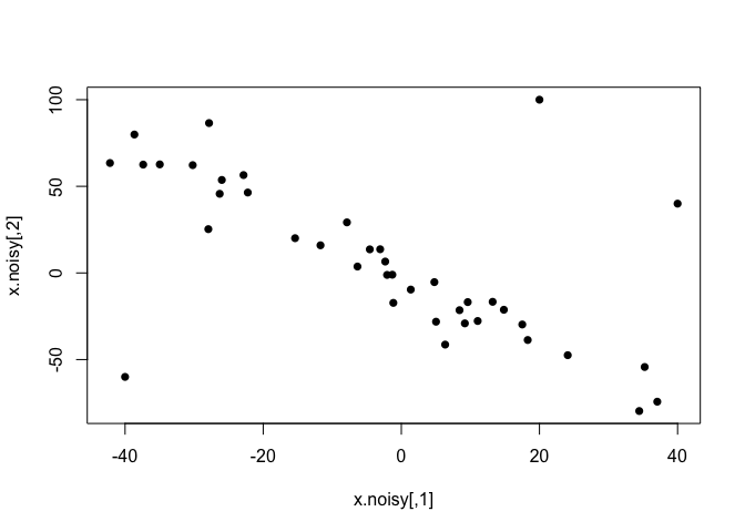
Now, classical methods are not happy with this kind of non-normal outliers, and both correlation coefficients decrease. While Pearson’s correlation is more sensitive, these outliers are extreme enough to have a large impact on Spearman’s as well.
cor(x.noisy, method="pearson")[1, 2]
## [1] -0.6365649
cor(x.noisy, method="spearman")[1, 2]
## [1] -0.6602251
As Bååth explained, we would like a model that is able to recognise the linear correlation in the bulk of the data, while accounting for the outliers as infrequent observations. The t-distribution does this naturally and dynamically, as long as we treat the degrees of freedom (nu) as a parameter with its own prior distribution.
The code for my initial Stan version of Bååth’s multivariate t model is shown below. I stuck pretty much to Bååth’s formulation, defining suitable noninformative priors for all model parameters; for the prior on nu, I followed the recommendation I found on John Kruschke’s blog.
data {
    int<lower=1> N;  // number of observations
    matrix[N, 2] x;  // input data: rows are observations, columns are the two variables
}

parameters {
    vector[2] mu;                 // locations of the marginal t distributions
    real<lower=0> sigma[2];       // scales of the marginal t distributions
    real<lower=0> nu;             // degrees of freedom of the marginal t distributions
    real<lower=-1, upper=1> rho;  // correlation coefficient
    vector[2] x_rand;             // random samples from the bivariate t distribution
}

transformed parameters {
    // Covariance matrix
    cov_matrix[2] cov = [[      sigma[1] ^ 2       , sigma[1] * sigma[2] * rho],
                         [sigma[1] * sigma[2] * rho,       sigma[2] ^ 2       ]];
}

model {
    // Likelihood
    // Bivariate Student's t-distribution instead of normal for robustness
    for (n in 1:N) {
        x[n] ~ multi_student_t(nu, mu, cov);
    }

    // Noninformative priors on all parameters
    sigma ~ uniform(0, 100000);
    rho ~ uniform(-1, 1);
    mu ~ normal(0, 100000);
    nu ~ exponential(1/30.0);

    // Draw samples from the estimated bivariate t-distribution (for assessment of fit)
    x_rand ~ multi_student_t(nu, mu, cov);
}
Now, although this initial model worked well (because of the relative simplicity of the problem), its performance could in fact be improved quite a bit. Soon after I posted a first version of this post on GitHub, Aki Vehtari himself kindly got in touch to recommend a series of valuable enhancements for the model, which are summarised below.
- Remove the
forloop in the likelihood to get 20x speedup (compute computationally costly common terms depending on nu, mu and sigma only once).- Generate
x_randin thegenerated quantitiesblock for extra speedup.- Don’t use
uniform()prior. It’s not needed forrho, which has implicit uniform prior on constrained range. Don’t use uniform to constrain parameters, so forsigmait’s better to use, e.g. half-normal.nubelow 1 is unlikely to be sensible, as then the distribution has no finite moments (except 0th moment), so use constraint<lower=1>.exponential(1/30)gives a lot of mass for very large values ofnu, I prefergamma(2,0.1), proposed and anlysed by Juárez and Steel (2010). See also this discussion.
As I agree that these changes should make the model faster and better behaved, I’m adopting this ‘Vehtarised’ model, which is reproduced below and can be found in the file robust_correlation.stan.
data {
    int<lower=1> N;  // number of observations
    vector[2] x[N];  // input data: rows are observations, columns are the two variables
}

parameters {
    vector[2] mu;                 // locations of the marginal t distributions
    real<lower=0> sigma[2];       // scales of the marginal t distributions
    real<lower=1> nu;             // degrees of freedom of the marginal t distributions
    real<lower=-1, upper=1> rho;  // correlation coefficient
}

transformed parameters {
    // Covariance matrix
    cov_matrix[2] cov = [[      sigma[1] ^ 2       , sigma[1] * sigma[2] * rho],
                         [sigma[1] * sigma[2] * rho,       sigma[2] ^ 2       ]];
}

model {
  // Likelihood
  // Bivariate Student's t-distribution instead of normal for robustness
  x ~ multi_student_t(nu, mu, cov);

  // Noninformative priors on all parameters
  sigma ~ normal(0,100);
  mu ~ normal(0, 100);
  nu ~ gamma(2, 0.1);
}

generated quantities {
  // Random samples from the estimated bivariate t-distribution (for assessment of fit)
  vector[2] x_rand;
  x_rand = multi_student_t_rng(nu, mu, cov);
}
Now, let’s first run the model on the clean data; the time this takes will depend on the number of iterations and chains we use, but it shouldn’t be long. The code below runs 4 independent MCMC chains (this is convenient in order to ensure that all the chains have converged to the same posterior distribution), with 2000 iterations per chain, the first 500 of which are warm-up iterations (these should cover the period when the MCMC chains are still converging, and so are discarded afterwards). We also set a seed for random number generation, to ensure that we obtain exactly the same output if we run the model multiple times.
(Note that the model has to be compiled the first time it is run. Some unimportant warning messages might show up during compilation, before MCMC sampling starts.)
# Set up model data
data.clean = list(x=x.clean, N=nrow(x.clean))

# Run the model
cor.clean = stan(file="robust_correlation.stan", data=data.clean,
                 iter=2000, warmup=500, chains=4, seed=210191)
##
## SAMPLING FOR MODEL 'robust_correlation' NOW (CHAIN 1).
##
## Gradient evaluation took 9.2e-05 seconds
## 1000 transitions using 10 leapfrog steps per transition would take 0.92 seconds.
## Adjust your expectations accordingly!
##
##
## Iteration:    1 / 2000 [  0%]  (Warmup)
## Iteration:  200 / 2000 [ 10%]  (Warmup)
## Iteration:  400 / 2000 [ 20%]  (Warmup)
## Iteration:  501 / 2000 [ 25%]  (Sampling)
## Iteration:  700 / 2000 [ 35%]  (Sampling)
## Iteration:  900 / 2000 [ 45%]  (Sampling)
## Iteration: 1100 / 2000 [ 55%]  (Sampling)
## Iteration: 1300 / 2000 [ 65%]  (Sampling)
## Iteration: 1500 / 2000 [ 75%]  (Sampling)
## Iteration: 1700 / 2000 [ 85%]  (Sampling)
## Iteration: 1900 / 2000 [ 95%]  (Sampling)
## Iteration: 2000 / 2000 [100%]  (Sampling)
##
##  Elapsed Time: 1.82912 seconds (Warm-up)
##                2.34811 seconds (Sampling)
##                4.17724 seconds (Total)
##
##
## SAMPLING FOR MODEL 'robust_correlation' NOW (CHAIN 2).
##
## Gradient evaluation took 9.2e-05 seconds
## 1000 transitions using 10 leapfrog steps per transition would take 0.92 seconds.
## Adjust your expectations accordingly!
##
##
## Iteration:    1 / 2000 [  0%]  (Warmup)
## Iteration:  200 / 2000 [ 10%]  (Warmup)
## Iteration:  400 / 2000 [ 20%]  (Warmup)
## Iteration:  501 / 2000 [ 25%]  (Sampling)
## Iteration:  700 / 2000 [ 35%]  (Sampling)
## Iteration:  900 / 2000 [ 45%]  (Sampling)
## Iteration: 1100 / 2000 [ 55%]  (Sampling)
## Iteration: 1300 / 2000 [ 65%]  (Sampling)
## Iteration: 1500 / 2000 [ 75%]  (Sampling)
## Iteration: 1700 / 2000 [ 85%]  (Sampling)
## Iteration: 1900 / 2000 [ 95%]  (Sampling)
## Iteration: 2000 / 2000 [100%]  (Sampling)
##
##  Elapsed Time: 1.79702 seconds (Warm-up)
##                2.69923 seconds (Sampling)
##                4.49625 seconds (Total)
##
##
## SAMPLING FOR MODEL 'robust_correlation' NOW (CHAIN 3).
##
## Gradient evaluation took 9.7e-05 seconds
## 1000 transitions using 10 leapfrog steps per transition would take 0.97 seconds.
## Adjust your expectations accordingly!
##
##
## Iteration:    1 / 2000 [  0%]  (Warmup)
## Iteration:  200 / 2000 [ 10%]  (Warmup)
## Iteration:  400 / 2000 [ 20%]  (Warmup)
## Iteration:  501 / 2000 [ 25%]  (Sampling)
## Iteration:  700 / 2000 [ 35%]  (Sampling)
## Iteration:  900 / 2000 [ 45%]  (Sampling)
## Iteration: 1100 / 2000 [ 55%]  (Sampling)
## Iteration: 1300 / 2000 [ 65%]  (Sampling)
## Iteration: 1500 / 2000 [ 75%]  (Sampling)
## Iteration: 1700 / 2000 [ 85%]  (Sampling)
## Iteration: 1900 / 2000 [ 95%]  (Sampling)
## Iteration: 2000 / 2000 [100%]  (Sampling)
##
##  Elapsed Time: 1.75095 seconds (Warm-up)
##                2.29858 seconds (Sampling)
##                4.04953 seconds (Total)
##
##
## SAMPLING FOR MODEL 'robust_correlation' NOW (CHAIN 4).
##
## Gradient evaluation took 0.000102 seconds
## 1000 transitions using 10 leapfrog steps per transition would take 1.02 seconds.
## Adjust your expectations accordingly!
##
##
## Iteration:    1 / 2000 [  0%]  (Warmup)
## Iteration:  200 / 2000 [ 10%]  (Warmup)
## Iteration:  400 / 2000 [ 20%]  (Warmup)
## Iteration:  501 / 2000 [ 25%]  (Sampling)
## Iteration:  700 / 2000 [ 35%]  (Sampling)
## Iteration:  900 / 2000 [ 45%]  (Sampling)
## Iteration: 1100 / 2000 [ 55%]  (Sampling)
## Iteration: 1300 / 2000 [ 65%]  (Sampling)
## Iteration: 1500 / 2000 [ 75%]  (Sampling)
## Iteration: 1700 / 2000 [ 85%]  (Sampling)
## Iteration: 1900 / 2000 [ 95%]  (Sampling)
## Iteration: 2000 / 2000 [100%]  (Sampling)
##
##  Elapsed Time: 1.69873 seconds (Warm-up)
##                2.40632 seconds (Sampling)
##                4.10505 seconds (Total)
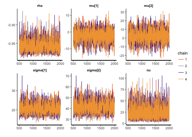
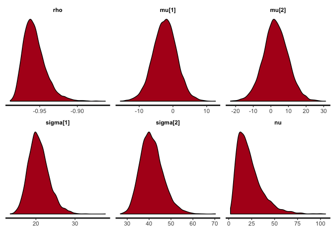
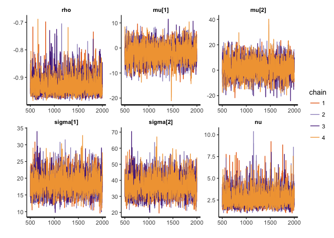
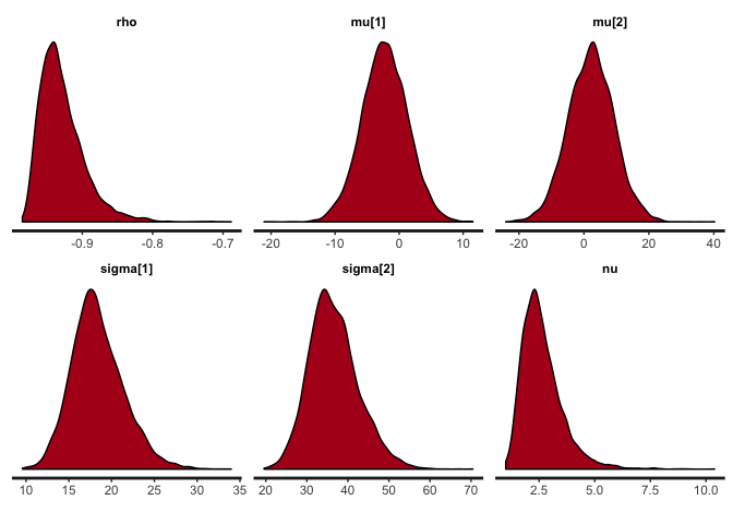
We can take a look at the MCMC traces and the inferred posterior distributions for rho (the correlation coefficient), mu, sigma (the locations and scales of the bivariate t-distribution), and nu (the degrees of freedom).
stan_trace(cor.clean, pars=c("rho", "mu", "sigma", "nu"))
stan_dens(cor.clean, pars=c("rho", "mu", "sigma", "nu"))
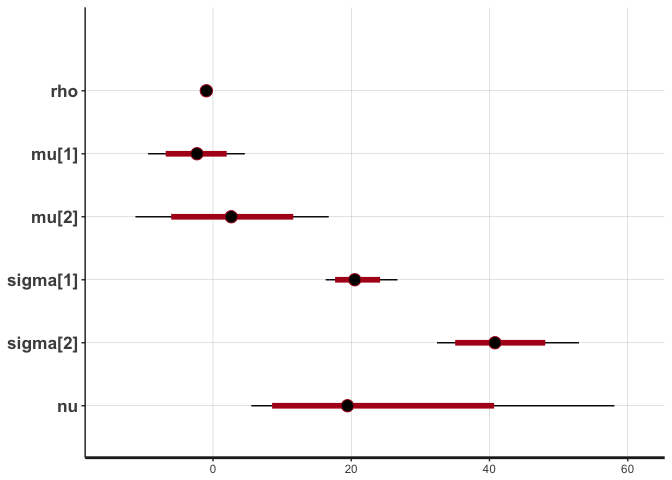
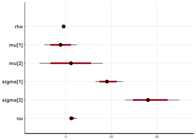
stan_plot(cor.clean, pars=c("rho", "mu", "sigma", "nu"))
## ci_level: 0.8 (80% intervals)

## outer_level: 0.95 (95% intervals)
The traces suggest convergence of the four MCMC chains, and almost all the weight of the posterior distribution of rho lies between -0.90 and -1. The posterior of nu covers large values, indicating that the data are normally distributed (remember that a t-distribution with high nu is equivalent to a normal distribution).
To make sure that the model is behaving well, we can take a look at the effective sample sizes and the values of the R-hat convergence statistic.
print(cor.clean)
## Inference for Stan model: robust_correlation.
## 4 chains, each with iter=2000; warmup=500; thin=1;
## post-warmup draws per chain=1500, total post-warmup draws=6000.
##
##              mean se_mean     sd     2.5%     25%     50%     75%   97.5%
## mu[1]       -2.38    0.06   3.53    -9.38   -4.69   -2.32   -0.07    4.61
## mu[2]        2.77    0.13   7.03   -11.21   -1.78    2.65    7.36   16.75
## sigma[1]    20.76    0.05   2.62    16.30   18.95   20.51   22.30   26.69
## sigma[2]    41.28    0.10   5.22    32.41   37.58   40.80   44.34   52.95
## nu          22.54    0.20  13.75     5.54   12.53   19.46   28.84   58.07
## rho         -0.96    0.00   0.02    -0.98   -0.97   -0.96   -0.95   -0.92
## cov[1,1]   437.72    2.31 113.23   265.84  359.11  420.73  497.19  712.50
## cov[1,2]  -833.68    4.53 219.90 -1359.78 -949.20 -801.37 -679.88 -500.54
## cov[2,1]  -833.68    4.53 219.90 -1359.78 -949.20 -801.37 -679.88 -500.54
## cov[2,2]  1731.00    8.99 448.04  1050.21 1412.30 1664.28 1966.46 2803.85
## x_rand[1]   -2.72    0.31  23.13   -49.01  -16.63   -2.34   11.57   42.48
## x_rand[2]    3.26    0.59  46.00   -86.15  -25.54    2.13   31.22   95.50
## lp__      -283.44    0.04   1.75  -287.59 -284.39 -283.12 -282.16 -281.00
##           n_eff Rhat
## mu[1]      3005    1
## mu[2]      2962    1
## sigma[1]   2447    1
## sigma[2]   2517    1
## nu         4552    1
## rho        3268    1
## cov[1,1]   2413    1
## cov[1,2]   2359    1
## cov[2,1]   2359    1
## cov[2,2]   2485    1
## x_rand[1]  5519    1
## x_rand[2]  6000    1
## lp__       2306    1
##
## Samples were drawn using NUTS(diag_e) at Mon May 28 17:36:39 2018.
## For each parameter, n_eff is a crude measure of effective sample size,
## and Rhat is the potential scale reduction factor on split chains (at
## convergence, Rhat=1).
The closer Rhat is to 1, the more confident we are that the MCMC chains have converged to the same distribution. The total number of post-warmup MCMC samples is 6000 (1500 per chain); the effective sample size (n_eff) gives the number of independent (i.e. non-autocorrelated) samples that these 6000 samples are equivalent to. In this case, all the effective sample sizes are above 2000, which is good enough for the purposes of this model.
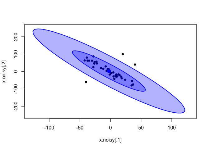
We can see how well the inferred bivariate distribution fits the data by plotting the random samples that the model drew from this distribution (x_rand in the model).
x.rand = extract(cor.clean, c("x_rand"))[[1]]
plot(x.clean, xlim=c(-60, 55), ylim=c(-120, 120), pch=16)
dataEllipse(x.rand, levels = c(0.5, 0.95),
            fill=T, plot.points = FALSE)
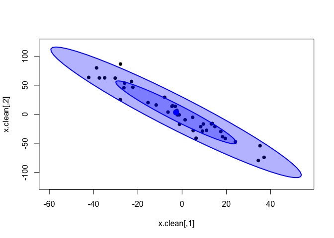
In the plot above, the dark-blue inner ellipse is the area containing 50% of the posterior distribution, and the pale-blue outer ellipse is the area containing 95% of the distribution.
It seems that the distribution inferred by the model does fit the data quite well. Now, this was expected for such eerily clean data. Let’s try on the noisy data; remember that the classical correlations were strongly affected by the introduced outliers.
cor(x.noisy, method="pearson")[1, 2]
## [1] -0.6365649
cor(x.noisy, method="spearman")[1, 2]
## [1] -0.6602251
We run the model on the noisy data as before.
# Set up model data
data.noisy = list(x=x.noisy, N=nrow(x.noisy))

# Run the model
cor.noisy = stan(file="robust_correlation.stan", data=data.noisy,
                 iter=2000, warmup=500, chains=4, seed=210191)
##
## SAMPLING FOR MODEL 'robust_correlation' NOW (CHAIN 1).
##
## Gradient evaluation took 0.000151 seconds
## 1000 transitions using 10 leapfrog steps per transition would take 1.51 seconds.
## Adjust your expectations accordingly!
##
##
## Iteration:    1 / 2000 [  0%]  (Warmup)
## Iteration:  200 / 2000 [ 10%]  (Warmup)
## Iteration:  400 / 2000 [ 20%]  (Warmup)
## Iteration:  501 / 2000 [ 25%]  (Sampling)
## Iteration:  700 / 2000 [ 35%]  (Sampling)
## Iteration:  900 / 2000 [ 45%]  (Sampling)
## Iteration: 1100 / 2000 [ 55%]  (Sampling)
## Iteration: 1300 / 2000 [ 65%]  (Sampling)
## Iteration: 1500 / 2000 [ 75%]  (Sampling)
## Iteration: 1700 / 2000 [ 85%]  (Sampling)
## Iteration: 1900 / 2000 [ 95%]  (Sampling)
## Iteration: 2000 / 2000 [100%]  (Sampling)
##
##  Elapsed Time: 1.54187 seconds (Warm-up)
##                1.91235 seconds (Sampling)
##                3.45421 seconds (Total)
##
##
## SAMPLING FOR MODEL 'robust_correlation' NOW (CHAIN 2).
##
## Gradient evaluation took 0.000149 seconds
## 1000 transitions using 10 leapfrog steps per transition would take 1.49 seconds.
## Adjust your expectations accordingly!
##
##
## Iteration:    1 / 2000 [  0%]  (Warmup)
## Iteration:  200 / 2000 [ 10%]  (Warmup)
## Iteration:  400 / 2000 [ 20%]  (Warmup)
## Iteration:  501 / 2000 [ 25%]  (Sampling)
## Iteration:  700 / 2000 [ 35%]  (Sampling)
## Iteration:  900 / 2000 [ 45%]  (Sampling)
## Iteration: 1100 / 2000 [ 55%]  (Sampling)
## Iteration: 1300 / 2000 [ 65%]  (Sampling)
## Iteration: 1500 / 2000 [ 75%]  (Sampling)
## Iteration: 1700 / 2000 [ 85%]  (Sampling)
## Iteration: 1900 / 2000 [ 95%]  (Sampling)
## Iteration: 2000 / 2000 [100%]  (Sampling)
##
##  Elapsed Time: 1.30011 seconds (Warm-up)
##                2.25888 seconds (Sampling)
##                3.559 seconds (Total)
##
##
## SAMPLING FOR MODEL 'robust_correlation' NOW (CHAIN 3).
##
## Gradient evaluation took 0.000204 seconds
## 1000 transitions using 10 leapfrog steps per transition would take 2.04 seconds.
## Adjust your expectations accordingly!
##
##
## Iteration:    1 / 2000 [  0%]  (Warmup)
## Iteration:  200 / 2000 [ 10%]  (Warmup)
## Iteration:  400 / 2000 [ 20%]  (Warmup)
## Iteration:  501 / 2000 [ 25%]  (Sampling)
## Iteration:  700 / 2000 [ 35%]  (Sampling)
## Iteration:  900 / 2000 [ 45%]  (Sampling)
## Iteration: 1100 / 2000 [ 55%]  (Sampling)
## Iteration: 1300 / 2000 [ 65%]  (Sampling)
## Iteration: 1500 / 2000 [ 75%]  (Sampling)
## Iteration: 1700 / 2000 [ 85%]  (Sampling)
## Iteration: 1900 / 2000 [ 95%]  (Sampling)
## Iteration: 2000 / 2000 [100%]  (Sampling)
##
##  Elapsed Time: 1.74736 seconds (Warm-up)
##                2.14554 seconds (Sampling)
##                3.8929 seconds (Total)
##
##
## SAMPLING FOR MODEL 'robust_correlation' NOW (CHAIN 4).
##
## Gradient evaluation took 0.000159 seconds
## 1000 transitions using 10 leapfrog steps per transition would take 1.59 seconds.
## Adjust your expectations accordingly!
##
##
## Iteration:    1 / 2000 [  0%]  (Warmup)
## Iteration:  200 / 2000 [ 10%]  (Warmup)
## Iteration:  400 / 2000 [ 20%]  (Warmup)
## Iteration:  501 / 2000 [ 25%]  (Sampling)
## Iteration:  700 / 2000 [ 35%]  (Sampling)
## Iteration:  900 / 2000 [ 45%]  (Sampling)
## Iteration: 1100 / 2000 [ 55%]  (Sampling)
## Iteration: 1300 / 2000 [ 65%]  (Sampling)
## Iteration: 1500 / 2000 [ 75%]  (Sampling)
## Iteration: 1700 / 2000 [ 85%]  (Sampling)
## Iteration: 1900 / 2000 [ 95%]  (Sampling)
## Iteration: 2000 / 2000 [100%]  (Sampling)
##
##  Elapsed Time: 1.46095 seconds (Warm-up)
##                2.07965 seconds (Sampling)
##                3.54059 seconds (Total)
# Plot traces and posteriors
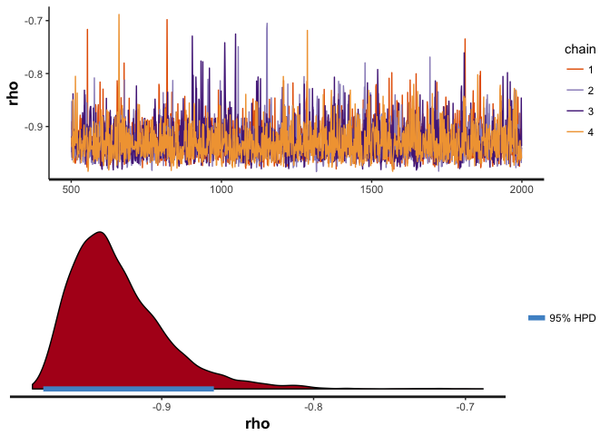
stan_trace(cor.noisy, pars=c("rho", "mu", "sigma", "nu"))
stan_dens(cor.noisy, pars=c("rho", "mu", "sigma", "nu"))
stan_plot(cor.noisy, pars=c("rho", "mu", "sigma", "nu"))
## ci_level: 0.8 (80% intervals)

## outer_level: 0.95 (95% intervals)
# Print statistics
print(cor.noisy)
## Inference for Stan model: robust_correlation.
## 4 chains, each with iter=2000; warmup=500; thin=1;
## post-warmup draws per chain=1500, total post-warmup draws=6000.
##
##              mean se_mean     sd     2.5%     25%     50%     75%   97.5%
## mu[1]       -2.23    0.07   3.58    -9.36   -4.58   -2.26    0.21    4.79
## mu[2]        2.21    0.14   7.07   -11.53   -2.53    2.30    6.97   16.28
## sigma[1]    18.37    0.06   3.05    13.01   16.29   18.05   20.21   25.05
## sigma[2]    36.59    0.12   6.04    26.00   32.44   36.05   40.18   49.72
## nu           2.64    0.02   0.93     1.37    2.01    2.47    3.07    4.95
## rho         -0.93    0.00   0.03    -0.97   -0.95   -0.94   -0.91   -0.85
## cov[1,1]   346.68    2.24 117.66   169.18  265.30  325.97  408.55  627.34
## cov[1,2]  -642.39    4.31 222.38 -1171.06 -757.64 -604.17 -489.07 -309.63
## cov[2,1]  -642.39    4.31 222.38 -1171.06 -757.64 -604.17 -489.07 -309.63
## cov[2,2]  1375.28    8.81 463.80   675.79 1052.21 1299.64 1614.06 2472.32
## x_rand[1]   -2.60    0.65  50.71   -70.81  -17.40   -2.26   12.03   65.79
## x_rand[2]    2.94    1.28  98.71  -132.58  -25.69    2.22   31.79  134.07
## lp__      -315.37    0.04   1.92  -320.00 -316.34 -314.99 -313.98 -312.84
##           n_eff Rhat
## mu[1]      2488    1
## mu[2]      2476    1
## sigma[1]   2537    1
## sigma[2]   2577    1
## nu         3733    1
## rho        3751    1
## cov[1,1]   2765    1
## cov[1,2]   2666    1
## cov[2,1]   2666    1
## cov[2,2]   2773    1
## x_rand[1]  6000    1
## x_rand[2]  5971    1
## lp__       1925    1
##
## Samples were drawn using NUTS(diag_e) at Mon May 28 17:36:57 2018.
## For each parameter, n_eff is a crude measure of effective sample size,
## and Rhat is the potential scale reduction factor on split chains (at
## convergence, Rhat=1).
The posterior distribution of rho hasn’t changed that much, but notice the difference in the posterior of nu. Lower values of nu indicate that the inferred bivariate t-distribution has heavy tails this time (i.e. is far from normality), in order to accommodate the outliers. If this noise were not accommodated in nu (e.g. if we used a normal distribution), then it would have to be accommodated in the distribution of rho, thus strongly biasing the correlation estimates.
Now, let’s see how the inferred bivariate t-distribution fits the noisy data.
x.rand = extract(cor.noisy, c("x_rand"))[[1]]
plot(x.noisy, xlim=c(-130, 130), ylim=c(-250, 250), pch=16)
dataEllipse(x.rand, levels = c(0.5, 0.95),
            fill=T, plot.points = FALSE)
The bivariate t-distribution seems to have a similar fit than the one inferred from the clean data; its slope is not affected by the outliers. However, notice how the tails of the distribution (pale-blue outer ellipse) have grown much larger than before.
Now that we have seen how the model provides robust estimation of the correlation coefficient, it would be good to take a good look at the estimated rho. Let’s extract the MCMC samples for this parameter’s posterior from the cor.noisy object produced by the stan function.
rho.noisy = as.numeric(extract(cor.noisy, "rho")[[1]])
length(rho.noisy)  # number of MCMC samples
## [1] 6000
median(rho.noisy) # posterior mean
## [1] -0.9350099
HPDinterval(as.mcmc(rho.noisy), prob=0.99) # 99% highest posterior density interval
##           lower      upper
## var1 -0.9846114 -0.8200769
## attr(,"Probability")
## [1] 0.99
rho has a posterior median of -0.935 and a 99% highest posterior density (HPD) interval of [-0.98, -0.82] (i.e. 99% of its posterior probability lies within this interval). The posterior median is very close to the original rho = -0.95 that we used to generate the data, reflecting the model’s robustness. But an important point here is that we can obtain these posterior statistics (and many more) by looking directly at the MCMC samples. Having direct access to the posterior distribution of the parameters we are interested in (in this case, the correlation coefficient) means that we don’t have to resort to null hypothesis testing to assess the certainty of our estimate.
For example, let’s run a standard correlation test on the noisy data.
cor.test(x.noisy[,1], x.noisy[,2], method="pearson")
##
##  Pearson's product-moment correlation
##
## data:  x.noisy[, 1] and x.noisy[, 2]
## t = -5.0881, df = 38, p-value = 1.008e-05
## alternative hypothesis: true correlation is not equal to 0
## 95 percent confidence interval:
##  -0.7911854 -0.4054558
## sample estimates:
##        cor
## -0.6365649
This provides the estimated value for the correlation coefficient (cor) together with a p-value and a confidence interval. In frequentist statistics, the estimated parameter is assumed to have a fixed, unknown true value, and this cor = -0.6365649 is the best informed guess of that value. The 95% confidence interval defines a range of likely values where the true value might be, but it is not the same as saying that this interval has a 95% probability of containing the true value; since the true value is assumed to be a fixed number, the probability of any interval containing the true value is either 0 or 1. The 95% confidence interval represents something more convoluted involving infinite hypothetical repetitions of the same analysis using different data samples.
The small p-value tells us what is the probability that values such as those in x.noisy, or even more strongly correlated, could be observed if the null hypothesis (that the true correlation is exactly zero) were correct. In other words, it’s the probability that the variables are not correlated in reality and what we are seeing is the product of random variation.
So, frequentist correlation tests have a rather indirect way of providing information about the true correlation coefficient. Let’s see now what we can say about this from the Bayesian standpoint. In Bayesian statistics, the true value of the parameter of interest is not a fixed quantity, but it has a probability distribution. We can investigate this distribution empirically simply by looking at the MCMC samples.
# Print some posterior statistics
# Posterior mean of rho
mean(rho.noisy)
## [1] -0.9286156
# Rho values with 99% posterior probability
hpd99 = HPDinterval(as.mcmc(rho.noisy), prob=0.99)
cat("[", hpd99[,"lower"], ", ", hpd99[,"upper"], "]", sep="")
## [-0.9846114, -0.8200769]
# Posterior probability that rho is ≤0, P(rho ≤ 0)
mean(rho.noisy <= 0)
## [1] 1
# Posterior probability that rho is ≥0, P(rho ≥ 0)
mean(rho.noisy >= 0)
## [1] 0
# Posterior probability that rho is <-0.5, P(rho < -0.5)
mean(rho.noisy < -0.5)
## [1] 1
# Posterior probability that rho is small, P(-0.1 < rho < 0.1)
mean(rho.noisy > -0.1 & rho.noisy < 0.1)
## [1] 0
This shows how we can directly interrogate the posterior distribution in order to make clear probabilistic statements about the distribution of the true rho. A statement like
According to the model, the correlation coefficient is between -0.83 and -0.98 with 99% probability
is somewhat more precise and clear than saying
According to the test, we are 95% confident that the correlation coefficient has a value somewhere between -0.41 and -0.79; we don’t really know if this interval contains the value, but if we could repeat this analysis on infinite different samples, we would be wrong just 5% of the time!
However, it is important to note that the precision of our posterior estimates will depend on how many iterations of MCMC sampling we perform. For example, note that the probability that rho is zero or positive, P(rho ≥ 0), is estimated to be zero. This statement is not entirely accurate, given that we didn’t run the model for very long. To increase the precision of our probabilistic statements, we would need to run the model for longer (i.e. sample more MCMC samples), and this would eventually give us a very small (but non-zero) posterior probability for this event. For example, if the actual posterior probability that rho is zero or positive were, say, one in a million, then we would need to sample (on average) a million MCMC samples in order to achieve the necessary accuracy. But normally we are not interested in that degree of precision; if we have sampled 6000 MCMC samples, we can at least declare the probability to be smaller than 1/6000.
Finally, I have wrapped the model itself and the code to run it inside a function called rob.cor.mcmc, which has optional arguments iter, warmup and chains for customised sampling, and can be found in the file rob.cor.mcmc.R. This function plots the MCMC trace and posterior distribution of rho, prints a handful of basic posterior statistics and returns the same object generated by the stan function (cor.noisy in the example above), from which you can then extract much more information using the rstan and coda packages.
# Now easier!
source("rob.cor.mcmc.R")
cor.noisy2 = rob.cor.mcmc(x.noisy)
##
## SAMPLING FOR MODEL 'robust_regression' NOW (CHAIN 1).
##
## Gradient evaluation took 8.6e-05 seconds
## 1000 transitions using 10 leapfrog steps per transition would take 0.86 seconds.
## Adjust your expectations accordingly!
##
##
## Iteration:    1 / 2000 [  0%]  (Warmup)
## Iteration:  200 / 2000 [ 10%]  (Warmup)
## Iteration:  400 / 2000 [ 20%]  (Warmup)
## Iteration:  501 / 2000 [ 25%]  (Sampling)
## Iteration:  700 / 2000 [ 35%]  (Sampling)
## Iteration:  900 / 2000 [ 45%]  (Sampling)
## Iteration: 1100 / 2000 [ 55%]  (Sampling)
## Iteration: 1300 / 2000 [ 65%]  (Sampling)
## Iteration: 1500 / 2000 [ 75%]  (Sampling)
## Iteration: 1700 / 2000 [ 85%]  (Sampling)
## Iteration: 1900 / 2000 [ 95%]  (Sampling)
## Iteration: 2000 / 2000 [100%]  (Sampling)
##
##  Elapsed Time: 1.50086 seconds (Warm-up)
##                1.82662 seconds (Sampling)
##                3.32749 seconds (Total)
##
##
## SAMPLING FOR MODEL 'robust_regression' NOW (CHAIN 2).
##
## Gradient evaluation took 7.8e-05 seconds
## 1000 transitions using 10 leapfrog steps per transition would take 0.78 seconds.
## Adjust your expectations accordingly!
##
##
## Iteration:    1 / 2000 [  0%]  (Warmup)
## Iteration:  200 / 2000 [ 10%]  (Warmup)
## Iteration:  400 / 2000 [ 20%]  (Warmup)
## Iteration:  501 / 2000 [ 25%]  (Sampling)
## Iteration:  700 / 2000 [ 35%]  (Sampling)
## Iteration:  900 / 2000 [ 45%]  (Sampling)
## Iteration: 1100 / 2000 [ 55%]  (Sampling)
## Iteration: 1300 / 2000 [ 65%]  (Sampling)
## Iteration: 1500 / 2000 [ 75%]  (Sampling)
## Iteration: 1700 / 2000 [ 85%]  (Sampling)
## Iteration: 1900 / 2000 [ 95%]  (Sampling)
## Iteration: 2000 / 2000 [100%]  (Sampling)
##
##  Elapsed Time: 1.19622 seconds (Warm-up)
##                2.17016 seconds (Sampling)
##                3.36638 seconds (Total)
##
##
## SAMPLING FOR MODEL 'robust_regression' NOW (CHAIN 3).
##
## Gradient evaluation took 8.7e-05 seconds
## 1000 transitions using 10 leapfrog steps per transition would take 0.87 seconds.
## Adjust your expectations accordingly!
##
##
## Iteration:    1 / 2000 [  0%]  (Warmup)
## Iteration:  200 / 2000 [ 10%]  (Warmup)
## Iteration:  400 / 2000 [ 20%]  (Warmup)
## Iteration:  501 / 2000 [ 25%]  (Sampling)
## Iteration:  700 / 2000 [ 35%]  (Sampling)
## Iteration:  900 / 2000 [ 45%]  (Sampling)
## Iteration: 1100 / 2000 [ 55%]  (Sampling)
## Iteration: 1300 / 2000 [ 65%]  (Sampling)
## Iteration: 1500 / 2000 [ 75%]  (Sampling)
## Iteration: 1700 / 2000 [ 85%]  (Sampling)
## Iteration: 1900 / 2000 [ 95%]  (Sampling)
## Iteration: 2000 / 2000 [100%]  (Sampling)
##
##  Elapsed Time: 1.67378 seconds (Warm-up)
##                1.99376 seconds (Sampling)
##                3.66754 seconds (Total)
##
##
## SAMPLING FOR MODEL 'robust_regression' NOW (CHAIN 4).
##
## Gradient evaluation took 8e-05 seconds
## 1000 transitions using 10 leapfrog steps per transition would take 0.8 seconds.
## Adjust your expectations accordingly!
##
##
## Iteration:    1 / 2000 [  0%]  (Warmup)
## Iteration:  200 / 2000 [ 10%]  (Warmup)
## Iteration:  400 / 2000 [ 20%]  (Warmup)
## Iteration:  501 / 2000 [ 25%]  (Sampling)
## Iteration:  700 / 2000 [ 35%]  (Sampling)
## Iteration:  900 / 2000 [ 45%]  (Sampling)
## Iteration: 1100 / 2000 [ 55%]  (Sampling)
## Iteration: 1300 / 2000 [ 65%]  (Sampling)
## Iteration: 1500 / 2000 [ 75%]  (Sampling)
## Iteration: 1700 / 2000 [ 85%]  (Sampling)
## Iteration: 1900 / 2000 [ 95%]  (Sampling)
## Iteration: 2000 / 2000 [100%]  (Sampling)
##
##  Elapsed Time: 1.39307 seconds (Warm-up)
##                2.0076 seconds (Sampling)
##                3.40067 seconds (Total)
## POSTERIOR STATISTICS OF RHO
## Posterior mean and standard deviation:     Mean = -0.9286156, SD = 0.03236113
## Posterior median and MAD:                  Median = -0.9350099, MAD = 0.02717319
## Rho values with 99% posterior probability: 99% HPDI = [-0.9846114, -0.8200769]
## Rho values with 95% posterior probability: 95% HPDI = [-0.9779942, -0.8656436]
## Posterior probability that rho is ≤0:      P(rho ≤ 0) = 1
## Posterior probability that rho is ≥0:      P(rho ≥ 0) = 0
## Posterior probability that rho is weak:    P(-0.1 < rho < 0.1) = 0
So, apart from having a sound statistical model that I can now use to estimate correlation in my noisy, noisy data, I will hopefully have convinced you (if you needed any convincing) of the potential of Bayesian methods for robust, flexible and clear data analysis.