Robust Bayesian linear regression with Stan in R
Adrian Baez-Ortega
6 August 2018
Simple linear regression is a very popular technique for estimating the linear relationship between two variables based on matched pairs of observations, as well as for predicting the probable value of one variable (the response variable) according to the value of the other (the explanatory variable). When plotting the results of linear regression graphically, the explanatory variable is normally plotted on the x-axis, and the response variable on the y-axis.
The standard approach to linear regression is defining the equation for a straight line that represents the relationship between the variables as accurately as possible. The equation for the line defines y (the response variable) as a linear function of x (the explanatory variable):
In this equation, ε represents the error in the linear relationship: if no noise were allowed, then the paired x- and y-values would need to be arranged in a perfect straight line (for example, as in y = 2x + 1). Because we assume that the relationship between x and y is truly linear, any variation observed around the regression line must be random noise, and therefore normally distributed. From a probabilistic standpoint, such relationship between the variables could be formalised as
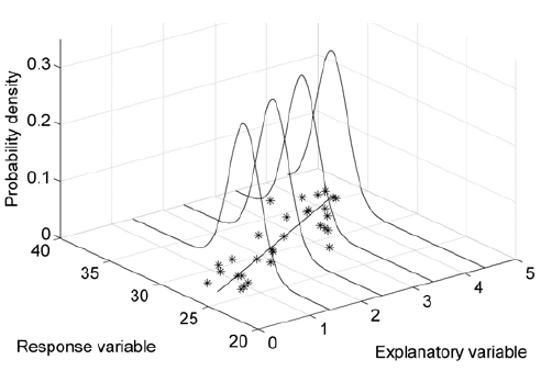
That is, the response variable follows a normal distribution with mean equal to the regression line, and some standard deviation σ. Such a probability distribution of the regression line is illustrated in the figure below.
This formulation inherently captures the random error around the regression line — as long as this error is normally distributed. Just as with Pearson’s correlation coefficient, the normality assumption adopted by classical regression methods makes them very sensitive to noisy or non-normal data. This frequently results in an underestimation of the relationship between the variables, as the normal distribution needs to shift its location in the parameter space in order to accommodate the outliers in the data as well as possible. In a frequentist paradigm, implementing a linear regression model that is robust to outliers entails quite convoluted statistical approaches; but in Bayesian statistics, when we need robustness, we just reach for the t-distribution. This probability distribution has a parameter ν, known as the degrees of freedom, which dictates how close to normality the distribution is: large values of ν (roughly ν > 30) result in a distribution that is very similar to the normal distribution, whereas low small values of ν produce a distribution with heavier tails (that is, a larger spread around the mean) than the normal distribution. Thus, by replacing the normal distribution above by a t-distribution, and incorporating ν as an extra parameter in the model, we can allow the distribution of the regression line to be as normal or non-normal as the data imply, while still capturing the underlying relationship between the variables.
The formulation of the robust simple linear regression Bayesian model is given below. We define a t likelihood for the response variable, y, and suitable vague priors on all the model parameters: normal for α and β, half-normal for σ and gamma for ν.
The Stan code for the model is reproduced below, and can be found in the file robust_regression.stan.
data {
    int<lower=1> N;    // number of observations
    int<lower=0> M;    // number of values for credible interval estimation
    int<lower=0> P;    // number of values to predict
    vector[N] x;       // input data for the explanatory (independent) variable
    vector[N] y;       // input data for the response (dependent) variable
    vector[M] x_cred;  // x-values for credible interval estimation (should cover range of x)
    vector[P] x_pred;  // x-values for prediction
}

parameters {
    real alpha;           // intercept
    real beta;            // coefficient
    real<lower=0> sigma;  // scale of the t-distribution
    real<lower=1> nu;     // degrees of freedom of the t-distribution
}

transformed parameters {
    vector[N] mu = alpha + beta * x;            // mean response
    vector[M] mu_cred = alpha + beta * x_cred;  // mean response for credible int. estimation
    vector[P] mu_pred = alpha + beta * x_pred;  // mean response for prediction
}

model {
    // Likelihood
    // Student's t-distribution instead of normal for robustness
    y ~ student_t(nu, mu, sigma);

    // Uninformative priors on all parameters
    alpha ~ normal(0, 1000);
    beta ~ normal(0, 1000);
    sigma ~ normal(0, 1000);
    nu ~ gamma(2, 0.1);
}

generated quantities {
    // Sample from the t-distribution at the values to predict (for prediction)
    real y_pred[P];
    for (p in 1:P) {
        y_pred[p] = student_t_rng(nu, mu_pred[p], sigma);
    }
}
Let’s pitch this Bayesian model against the standard linear model fitting provided in R (lm function) on some simulated data. We will need the following packages:
library(rstan)    # to run the Bayesian model (stan)
library(coda)     # to obtain HPD intervals (HPDinterval)
library(mvtnorm)  # to generate random correlated data (rmvnorm)
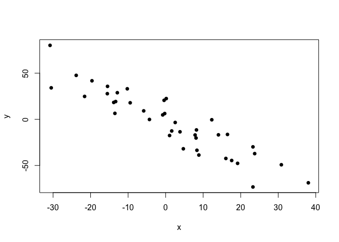
We can generate random data from a multivariate normal distribution with pre-specified correlation (rho) using the rmvnorm function in the mvtnorm package.
sigma = c(20, 40)
rho = -0.95
cov.mat = matrix(c(sigma[1] ^ 2,
                   sigma[1] * sigma[2] * rho,
                   sigma[1] * sigma[2] * rho,
                   sigma[2] ^ 2),
                 nrow=2, byrow=T)

set.seed(191)
points.clean = as.data.frame(rmvnorm(n=40, sigma=cov.mat))
colnames(points.clean) = c("x", "y")
plot(points.clean, pch=16)
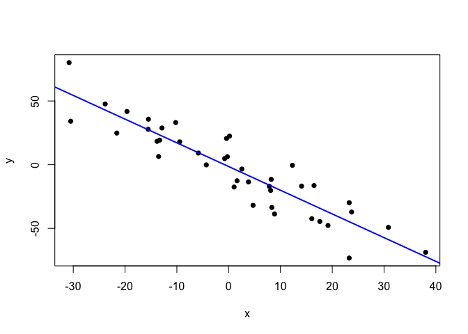
Let’s first run the standard lm function on these data and look at the fit.
lm.fit.clean = lm(y ~ x, data=points.clean)
plot(points.clean, pch=16)
abline(lm.fit.clean, col="blue", lwd=2)
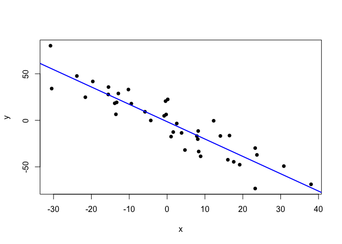
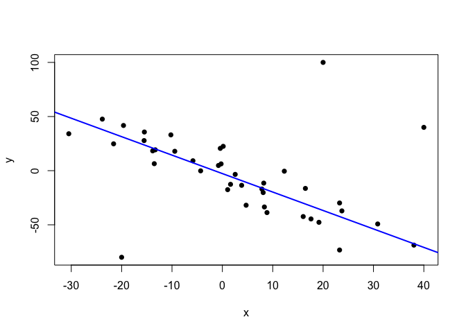
Quite publication-ready. But, since these data are somewhat too clean for my taste, let’s sneak some extreme outliers in.
points.noisy = points.clean
points.noisy[1:3,] = matrix(c(-20, -80,
                              20, 100,
                              40, 40),
                            nrow=3, byrow=T)
plot(points.noisy, pch=16)
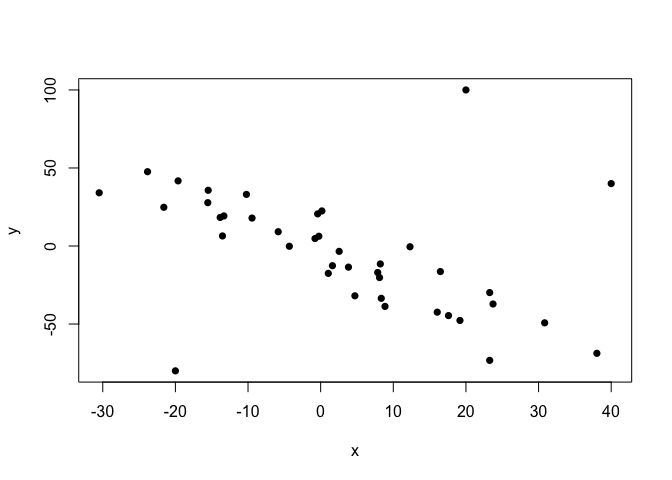
Now, the normally-distributed-error assumption of the standard linear regression model doesn’t deal well with this kind of non-normal outliers (as they indeed break the model’s assumption), and so the estimated regression line comes to a disagreement with the relationship displayed by the bulk of the data points.
lm.fit.noisy = lm(y ~ x, data=points.noisy)
plot(points.noisy, pch=16)
abline(lm.fit.noisy, col="blue", lwd=2)
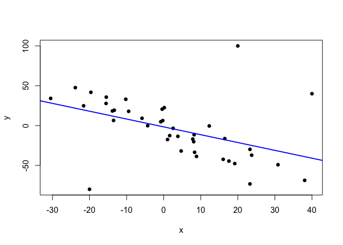
Thus, we need a model that is able to recognise the linear relationship present in the data, while accounting the outliers as infrequent, atypical observations. The t-distribution does this naturally and dynamically, as long as we treat the degrees of freedom, ν, as a parameter with its own prior distribution.
So, let’s now run our Bayesian regression model on the clean data first. The time this takes will depend on the number of iterations and chains we use, but it shouldn’t be long. (Note that the model has to be compiled the first time it is run. Some unimportant warning messages might show up during compilation, before MCMC sampling starts.)
# Set up model data
# As we are not going to build credible or prediction intervals yet,
# we will not use M, P, x_cred and x_pred
data.clean = list(x=points.clean$x,
                  y=points.clean$y,
                  N=nrow(points.clean),
                  M=0, P=0, x_cred=numeric(0), x_pred=numeric(0))

# Run the model
reg.clean = stan(file="robust_regression.stan", data=data.clean,
                 iter=1000, warmup=500, chains=4, seed=210191)
##
## SAMPLING FOR MODEL 'robust_regression' NOW (CHAIN 1).
##
## Gradient evaluation took 1.2e-05 seconds
## 1000 transitions using 10 leapfrog steps per transition would take 0.12 seconds.
## Adjust your expectations accordingly!
##
##
## Iteration:   1 / 1000 [  0%]  (Warmup)
## Iteration: 100 / 1000 [ 10%]  (Warmup)
## Iteration: 200 / 1000 [ 20%]  (Warmup)
## Iteration: 300 / 1000 [ 30%]  (Warmup)
## Iteration: 400 / 1000 [ 40%]  (Warmup)
## Iteration: 500 / 1000 [ 50%]  (Warmup)
## Iteration: 501 / 1000 [ 50%]  (Sampling)
## Iteration: 600 / 1000 [ 60%]  (Sampling)
## Iteration: 700 / 1000 [ 70%]  (Sampling)
## Iteration: 800 / 1000 [ 80%]  (Sampling)
## Iteration: 900 / 1000 [ 90%]  (Sampling)
## Iteration: 1000 / 1000 [100%]  (Sampling)
##
##  Elapsed Time: 0.039895 seconds (Warm-up)
##                0.026191 seconds (Sampling)
##                0.066086 seconds (Total)
##
##
## SAMPLING FOR MODEL 'robust_regression' NOW (CHAIN 2).
##
## Gradient evaluation took 1.5e-05 seconds
## 1000 transitions using 10 leapfrog steps per transition would take 0.15 seconds.
## Adjust your expectations accordingly!
##
##
## Iteration:   1 / 1000 [  0%]  (Warmup)
## Iteration: 100 / 1000 [ 10%]  (Warmup)
## Iteration: 200 / 1000 [ 20%]  (Warmup)
## Iteration: 300 / 1000 [ 30%]  (Warmup)
## Iteration: 400 / 1000 [ 40%]  (Warmup)
## Iteration: 500 / 1000 [ 50%]  (Warmup)
## Iteration: 501 / 1000 [ 50%]  (Sampling)
## Iteration: 600 / 1000 [ 60%]  (Sampling)
## Iteration: 700 / 1000 [ 70%]  (Sampling)
## Iteration: 800 / 1000 [ 80%]  (Sampling)
## Iteration: 900 / 1000 [ 90%]  (Sampling)
## Iteration: 1000 / 1000 [100%]  (Sampling)
##
##  Elapsed Time: 0.039082 seconds (Warm-up)
##                0.026199 seconds (Sampling)
##                0.065281 seconds (Total)
##
##
## SAMPLING FOR MODEL 'robust_regression' NOW (CHAIN 3).
##
## Gradient evaluation took 1.2e-05 seconds
## 1000 transitions using 10 leapfrog steps per transition would take 0.12 seconds.
## Adjust your expectations accordingly!
##
##
## Iteration:   1 / 1000 [  0%]  (Warmup)
## Iteration: 100 / 1000 [ 10%]  (Warmup)
## Iteration: 200 / 1000 [ 20%]  (Warmup)
## Iteration: 300 / 1000 [ 30%]  (Warmup)
## Iteration: 400 / 1000 [ 40%]  (Warmup)
## Iteration: 500 / 1000 [ 50%]  (Warmup)
## Iteration: 501 / 1000 [ 50%]  (Sampling)
## Iteration: 600 / 1000 [ 60%]  (Sampling)
## Iteration: 700 / 1000 [ 70%]  (Sampling)
## Iteration: 800 / 1000 [ 80%]  (Sampling)
## Iteration: 900 / 1000 [ 90%]  (Sampling)
## Iteration: 1000 / 1000 [100%]  (Sampling)
##
##  Elapsed Time: 0.042808 seconds (Warm-up)
##                0.023388 seconds (Sampling)
##                0.066196 seconds (Total)
##
##
## SAMPLING FOR MODEL 'robust_regression' NOW (CHAIN 4).
##
## Gradient evaluation took 1.4e-05 seconds
## 1000 transitions using 10 leapfrog steps per transition would take 0.14 seconds.
## Adjust your expectations accordingly!
##
##
## Iteration:   1 / 1000 [  0%]  (Warmup)
## Iteration: 100 / 1000 [ 10%]  (Warmup)
## Iteration: 200 / 1000 [ 20%]  (Warmup)
## Iteration: 300 / 1000 [ 30%]  (Warmup)
## Iteration: 400 / 1000 [ 40%]  (Warmup)
## Iteration: 500 / 1000 [ 50%]  (Warmup)
## Iteration: 501 / 1000 [ 50%]  (Sampling)
## Iteration: 600 / 1000 [ 60%]  (Sampling)
## Iteration: 700 / 1000 [ 70%]  (Sampling)
## Iteration: 800 / 1000 [ 80%]  (Sampling)
## Iteration: 900 / 1000 [ 90%]  (Sampling)
## Iteration: 1000 / 1000 [100%]  (Sampling)
##
##  Elapsed Time: 0.035621 seconds (Warm-up)
##                0.029625 seconds (Sampling)
##                0.065246 seconds (Total)
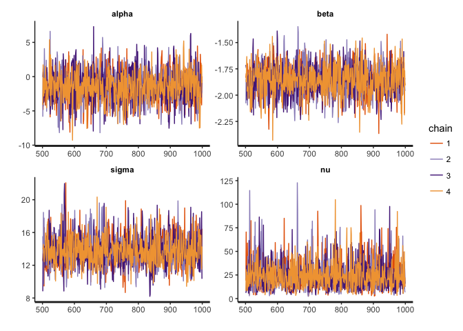
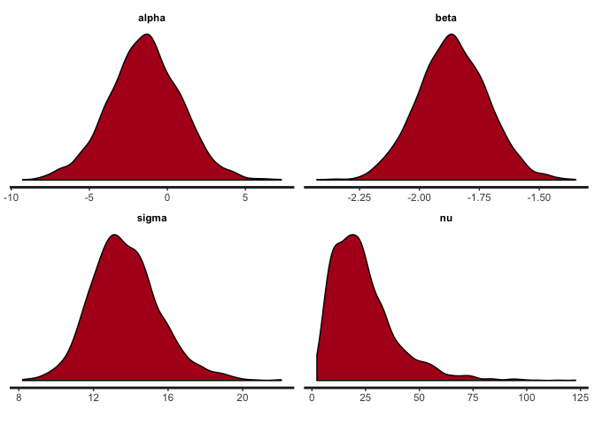
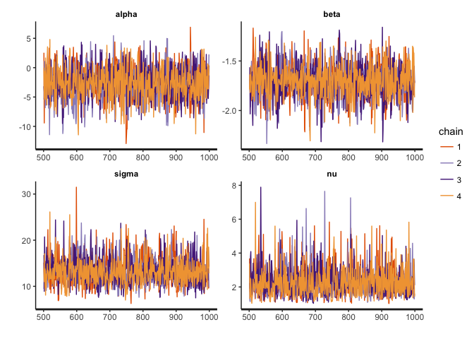
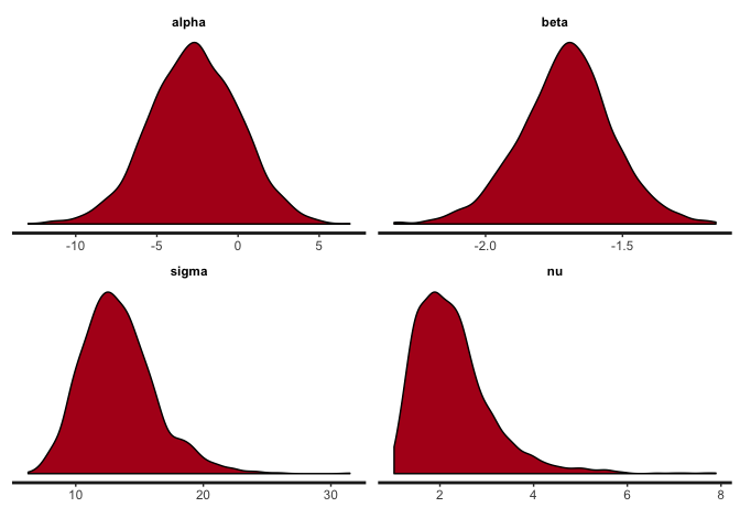
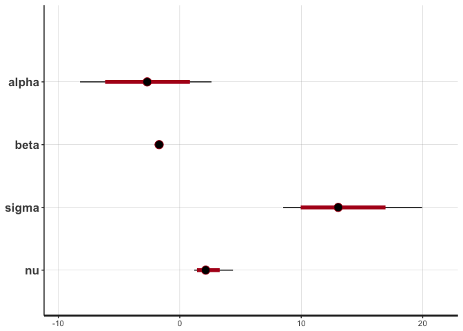
We can take a look at the MCMC traces and the posterior distributions for alpha, beta (the intercept and slope of the regression line), sigma and nu (the spread and degrees of freedom of the t-distribution).
stan_trace(reg.clean, pars=c("alpha", "beta", "sigma", "nu"))
stan_dens(reg.clean, pars=c("alpha", "beta", "sigma", "nu"))
stan_plot(reg.clean, pars=c("alpha", "beta", "sigma", "nu"))
## ci_level: 0.8 (80% intervals)

## outer_level: 0.95 (95% intervals)
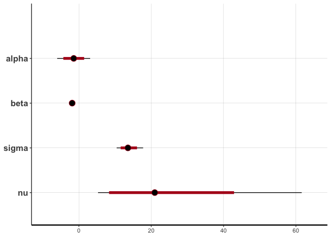
The traces show convergence of the four MCMC chains to the same distribution for each parameter, and we can see that the posterior of nu covers relatively large values, indicating that the data are normally distributed (remember that a t-distribution with high nu is equivalent to a normal distribution).
Let’s plot the regression line from this model, using the posterior mean estimates of alpha and beta.
alpha.clean = mean(extract(reg.clean, "alpha")[[1]])
beta.clean = mean(extract(reg.clean, "beta")[[1]])

plot(points.clean, pch=16)
abline(alpha.clean, beta.clean, col="blue", lwd=2)
We can see that the model fits the normally distributed data just as well as the standard linear regression model. However, the difference lies in how this model behaves when faced with the noisy, non-normal data.
# Set up model data
# As we are not going to build credible or prediction intervals yet,
# we will not use M, P, x_cred and x_pred
data.noisy = list(x=points.noisy$x,
                  y=points.noisy$y,
                  N=nrow(points.noisy),
                  M=0, P=0, x_cred=numeric(0), x_pred=numeric(0))

# Run the model
reg.noisy = stan(file="robust_regression.stan", data=data.noisy,
                 iter=1000, warmup=500, chains=4, seed=210191)
##
## SAMPLING FOR MODEL 'robust_regression' NOW (CHAIN 1).
##
## Gradient evaluation took 1.3e-05 seconds
## 1000 transitions using 10 leapfrog steps per transition would take 0.13 seconds.
## Adjust your expectations accordingly!
##
##
## Iteration:   1 / 1000 [  0%]  (Warmup)
## Iteration: 100 / 1000 [ 10%]  (Warmup)
## Iteration: 200 / 1000 [ 20%]  (Warmup)
## Iteration: 300 / 1000 [ 30%]  (Warmup)
## Iteration: 400 / 1000 [ 40%]  (Warmup)
## Iteration: 500 / 1000 [ 50%]  (Warmup)
## Iteration: 501 / 1000 [ 50%]  (Sampling)
## Iteration: 600 / 1000 [ 60%]  (Sampling)
## Iteration: 700 / 1000 [ 70%]  (Sampling)
## Iteration: 800 / 1000 [ 80%]  (Sampling)
## Iteration: 900 / 1000 [ 90%]  (Sampling)
## Iteration: 1000 / 1000 [100%]  (Sampling)
##
##  Elapsed Time: 0.038151 seconds (Warm-up)
##                0.024285 seconds (Sampling)
##                0.062436 seconds (Total)
##
##
## SAMPLING FOR MODEL 'robust_regression' NOW (CHAIN 2).
##
## Gradient evaluation took 1.3e-05 seconds
## 1000 transitions using 10 leapfrog steps per transition would take 0.13 seconds.
## Adjust your expectations accordingly!
##
##
## Iteration:   1 / 1000 [  0%]  (Warmup)
## Iteration: 100 / 1000 [ 10%]  (Warmup)
## Iteration: 200 / 1000 [ 20%]  (Warmup)
## Iteration: 300 / 1000 [ 30%]  (Warmup)
## Iteration: 400 / 1000 [ 40%]  (Warmup)
## Iteration: 500 / 1000 [ 50%]  (Warmup)
## Iteration: 501 / 1000 [ 50%]  (Sampling)
## Iteration: 600 / 1000 [ 60%]  (Sampling)
## Iteration: 700 / 1000 [ 70%]  (Sampling)
## Iteration: 800 / 1000 [ 80%]  (Sampling)
## Iteration: 900 / 1000 [ 90%]  (Sampling)
## Iteration: 1000 / 1000 [100%]  (Sampling)
##
##  Elapsed Time: 0.040687 seconds (Warm-up)
##                0.023764 seconds (Sampling)
##                0.064451 seconds (Total)
##
##
## SAMPLING FOR MODEL 'robust_regression' NOW (CHAIN 3).
##
## Gradient evaluation took 1e-05 seconds
## 1000 transitions using 10 leapfrog steps per transition would take 0.1 seconds.
## Adjust your expectations accordingly!
##
##
## Iteration:   1 / 1000 [  0%]  (Warmup)
## Iteration: 100 / 1000 [ 10%]  (Warmup)
## Iteration: 200 / 1000 [ 20%]  (Warmup)
## Iteration: 300 / 1000 [ 30%]  (Warmup)
## Iteration: 400 / 1000 [ 40%]  (Warmup)
## Iteration: 500 / 1000 [ 50%]  (Warmup)
## Iteration: 501 / 1000 [ 50%]  (Sampling)
## Iteration: 600 / 1000 [ 60%]  (Sampling)
## Iteration: 700 / 1000 [ 70%]  (Sampling)
## Iteration: 800 / 1000 [ 80%]  (Sampling)
## Iteration: 900 / 1000 [ 90%]  (Sampling)
## Iteration: 1000 / 1000 [100%]  (Sampling)
##
##  Elapsed Time: 0.039823 seconds (Warm-up)
##                0.023893 seconds (Sampling)
##                0.063716 seconds (Total)
##
##
## SAMPLING FOR MODEL 'robust_regression' NOW (CHAIN 4).
##
## Gradient evaluation took 1.7e-05 seconds
## 1000 transitions using 10 leapfrog steps per transition would take 0.17 seconds.
## Adjust your expectations accordingly!
##
##
## Iteration:   1 / 1000 [  0%]  (Warmup)
## Iteration: 100 / 1000 [ 10%]  (Warmup)
## Iteration: 200 / 1000 [ 20%]  (Warmup)
## Iteration: 300 / 1000 [ 30%]  (Warmup)
## Iteration: 400 / 1000 [ 40%]  (Warmup)
## Iteration: 500 / 1000 [ 50%]  (Warmup)
## Iteration: 501 / 1000 [ 50%]  (Sampling)
## Iteration: 600 / 1000 [ 60%]  (Sampling)
## Iteration: 700 / 1000 [ 70%]  (Sampling)
## Iteration: 800 / 1000 [ 80%]  (Sampling)
## Iteration: 900 / 1000 [ 90%]  (Sampling)
## Iteration: 1000 / 1000 [100%]  (Sampling)
##
##  Elapsed Time: 0.037346 seconds (Warm-up)
##                0.022237 seconds (Sampling)
##                0.059583 seconds (Total)
stan_trace(reg.noisy, pars=c("alpha", "beta", "sigma", "nu"))
stan_dens(reg.noisy, pars=c("alpha", "beta", "sigma", "nu"))
stan_plot(reg.noisy, pars=c("alpha", "beta", "sigma", "nu"))
## ci_level: 0.8 (80% intervals)

## outer_level: 0.95 (95% intervals)
The posteriors of alpha, beta and sigma haven’t changed that much, but notice the difference in the posterior of nu. Lower values of nu indicate that the t-distribution has heavy tails this time, in order to accommodate the outliers. If the noise introduced by the outliers were not accommodated in nu (that is, if we used a normal distribution), then it would have to be accommodated in the other parameters, resulting in a deviated regression line like the one estimated by the lm function.
Let’s look at the regression line:
alpha.noisy = mean(extract(reg.noisy, "alpha")[[1]])
beta.noisy = mean(extract(reg.noisy, "beta")[[1]])

plot(points.noisy, pch=16)
abline(alpha.noisy, beta.noisy, col="blue", lwd=2)
The line seems to be right on the spot. In fact, let’s compare it with the line inferred from the clean data by our model, and with the line estimated by the conventional linear model (lm).
plot(points.noisy, pch=16)
abline(lm.fit.noisy, col="orange", lwd=2)
abline(alpha.clean, beta.clean, col="red", lwd=2)
abline(alpha.noisy, beta.noisy, col="blue", lwd=2)
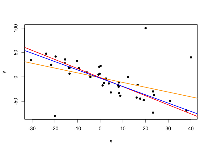
The line inferred by the Bayesian model from the noisy data (blue) reveals only a moderate influence of the outliers when compared to the line inferred from the clean data (red). However, the effect of the outliers is much more severe in the line inferred by the lm function from the noisy data (orange).
Just as conventional regression models, our Bayesian model can be used to estimate credible (or highest posterior density) intervals for the mean response (that is, intervals summarising the distribution of the regression line), and prediction intervals, by using the model’s predictive posterior distributions. More specifically, the credible intervals are obtained by drawing MCMC samples of the mean response (mu_cred = alpha + beta * x_cred) at regularly spaced points along the x-axis (x_cred), while the prediction intervals are obtained by first drawing samples of the mean response (mu_pred) at particular x-values of interest (x_pred), and then, for each of these samples, drawing a random y-value (y_pred) from a t-distribution with location mu_pred (see the model code above). The credible and prediction intervals reflect the distributions of mu_cred and y_pred, respectively.
That said, the truth is that getting prediction intervals from our model is as simple as using x_cred to specify a sequence of values spanning the range of the x-values in the data. We’ll also take the opportunity to obtain prediction intervals for a couple of arbitrary x-values.
# Define a sequence of x values for the credible intervals
x.cred = seq(from=min(points.noisy$x),
             to=max(points.noisy$x),
             length.out=20)
x.cred
##  [1] -30.4893736 -26.7794066 -23.0694396 -19.3594725 -15.6495055
##  [6] -11.9395385  -8.2295714  -4.5196044  -0.8096374   2.9003297
## [11]   6.6102967  10.3202637  14.0302308  17.7401978  21.4501648
## [16]  25.1601319  28.8700989  32.5800659  36.2900330  40.0000000
# Define x values whose response is to be predicted
x.pred = c(-25, 30)

# Set up model data
data.noisy2 = list(x=points.noisy$x,
                   y=points.noisy$y,
                   x_cred=x.cred,
                   x_pred=x.pred,
                   N=nrow(points.noisy),
                   M=length(x.cred),
                   P=length(x.pred))

# Run the model
reg.noisy2 = stan(file="robust_regression.stan", data=data.noisy2,
                  iter=3000, warmup=1000, chains=4, seed=210191)
##
## SAMPLING FOR MODEL 'robust_regression' NOW (CHAIN 1).
##
## Gradient evaluation took 1.5e-05 seconds
## 1000 transitions using 10 leapfrog steps per transition would take 0.15 seconds.
## Adjust your expectations accordingly!
##
##
## Iteration:    1 / 3000 [  0%]  (Warmup)
## Iteration:  300 / 3000 [ 10%]  (Warmup)
## Iteration:  600 / 3000 [ 20%]  (Warmup)
## Iteration:  900 / 3000 [ 30%]  (Warmup)
## Iteration: 1001 / 3000 [ 33%]  (Sampling)
## Iteration: 1300 / 3000 [ 43%]  (Sampling)
## Iteration: 1600 / 3000 [ 53%]  (Sampling)
## Iteration: 1900 / 3000 [ 63%]  (Sampling)
## Iteration: 2200 / 3000 [ 73%]  (Sampling)
## Iteration: 2500 / 3000 [ 83%]  (Sampling)
## Iteration: 2800 / 3000 [ 93%]  (Sampling)
## Iteration: 3000 / 3000 [100%]  (Sampling)
##
##  Elapsed Time: 0.077028 seconds (Warm-up)
##                0.121909 seconds (Sampling)
##                0.198937 seconds (Total)
##
##
## SAMPLING FOR MODEL 'robust_regression' NOW (CHAIN 2).
##
## Gradient evaluation took 1.5e-05 seconds
## 1000 transitions using 10 leapfrog steps per transition would take 0.15 seconds.
## Adjust your expectations accordingly!
##
##
## Iteration:    1 / 3000 [  0%]  (Warmup)
## Iteration:  300 / 3000 [ 10%]  (Warmup)
## Iteration:  600 / 3000 [ 20%]  (Warmup)
## Iteration:  900 / 3000 [ 30%]  (Warmup)
## Iteration: 1001 / 3000 [ 33%]  (Sampling)
## Iteration: 1300 / 3000 [ 43%]  (Sampling)
## Iteration: 1600 / 3000 [ 53%]  (Sampling)
## Iteration: 1900 / 3000 [ 63%]  (Sampling)
## Iteration: 2200 / 3000 [ 73%]  (Sampling)
## Iteration: 2500 / 3000 [ 83%]  (Sampling)
## Iteration: 2800 / 3000 [ 93%]  (Sampling)
## Iteration: 3000 / 3000 [100%]  (Sampling)
##
##  Elapsed Time: 0.079265 seconds (Warm-up)
##                0.12608 seconds (Sampling)
##                0.205345 seconds (Total)
##
##
## SAMPLING FOR MODEL 'robust_regression' NOW (CHAIN 3).
##
## Gradient evaluation took 1.3e-05 seconds
## 1000 transitions using 10 leapfrog steps per transition would take 0.13 seconds.
## Adjust your expectations accordingly!
##
##
## Iteration:    1 / 3000 [  0%]  (Warmup)
## Iteration:  300 / 3000 [ 10%]  (Warmup)
## Iteration:  600 / 3000 [ 20%]  (Warmup)
## Iteration:  900 / 3000 [ 30%]  (Warmup)
## Iteration: 1001 / 3000 [ 33%]  (Sampling)
## Iteration: 1300 / 3000 [ 43%]  (Sampling)
## Iteration: 1600 / 3000 [ 53%]  (Sampling)
## Iteration: 1900 / 3000 [ 63%]  (Sampling)
## Iteration: 2200 / 3000 [ 73%]  (Sampling)
## Iteration: 2500 / 3000 [ 83%]  (Sampling)
## Iteration: 2800 / 3000 [ 93%]  (Sampling)
## Iteration: 3000 / 3000 [100%]  (Sampling)
##
##  Elapsed Time: 0.08802 seconds (Warm-up)
##                0.127249 seconds (Sampling)
##                0.215269 seconds (Total)
##
##
## SAMPLING FOR MODEL 'robust_regression' NOW (CHAIN 4).
##
## Gradient evaluation took 1.6e-05 seconds
## 1000 transitions using 10 leapfrog steps per transition would take 0.16 seconds.
## Adjust your expectations accordingly!
##
##
## Iteration:    1 / 3000 [  0%]  (Warmup)
## Iteration:  300 / 3000 [ 10%]  (Warmup)
## Iteration:  600 / 3000 [ 20%]  (Warmup)
## Iteration:  900 / 3000 [ 30%]  (Warmup)
## Iteration: 1001 / 3000 [ 33%]  (Sampling)
## Iteration: 1300 / 3000 [ 43%]  (Sampling)
## Iteration: 1600 / 3000 [ 53%]  (Sampling)
## Iteration: 1900 / 3000 [ 63%]  (Sampling)
## Iteration: 2200 / 3000 [ 73%]  (Sampling)
## Iteration: 2500 / 3000 [ 83%]  (Sampling)
## Iteration: 2800 / 3000 [ 93%]  (Sampling)
## Iteration: 3000 / 3000 [100%]  (Sampling)
##
##  Elapsed Time: 0.08512 seconds (Warm-up)
##                0.138439 seconds (Sampling)
##                0.223559 seconds (Total)
Let’s see those credible intervals; in fact, we’ll plot highest posterior density (HPD) intervals instead of credible intervals, as they are more informative and easy to obtain with the coda package.
alpha.noisy = mean(extract(reg.noisy2, "alpha")[[1]])
beta.noisy = mean(extract(reg.noisy2, "beta")[[1]])
mu.cred = extract(reg.noisy2, "mu_cred")[[1]]
dim(mu.cred)
## [1] 8000 20
y.pred = extract(reg.noisy2, "y_pred")[[1]]
dim(y.pred)
## [1] 8000 2
Each column of mu.cred contains the MCMC samples of the mu_cred parameter (the posterior mean response) for each of the 20 x-values in x.cred. Similarly, the columns of y.pred contain the MCMC samples of the randomly drawn y_pred values (posterior predicted response values) for the x-values in x.pred. What we need are the HPD intervals derived from each column, which will give us the higher and lower ends of the interval to plot at each point. We will also calculate the column medians of y.pred, which serve as posterior point estimates of the predicted response for the values in x.pred (such estimates should lie on the estimated regression line, as this represents the predicted mean response).
mu.cred.hpd = apply(mu.cred, 2, function(mu) HPDinterval(as.mcmc(mu)))
mu.cred.hpd
##
## iterations     [,1]     [,2]     [,3]     [,4]     [,5]     [,6]      [,7]
##       [1,] 37.80837 32.34207 26.88122 21.63776 16.05987 10.85247  5.144538
##       [2,] 61.42437 53.94797 46.35011 39.05369 31.50101 24.51414 17.334380
##
## iterations       [,8]      [,9]      [,10]      [,11]     [,12]     [,13]
##       [1,] -0.5950497 -6.296941 -12.562931 -19.210834 -26.31466 -32.81720
##       [2,] 10.5850896  4.204336  -2.160792  -8.247743 -14.20289 -19.25666
##
## iterations     [,14]     [,15]     [,16]     [,17]     [,18]     [,19]
##       [1,] -40.15208 -47.47240 -55.21318 -62.63669 -69.91902 -77.18323
##       [2,] -24.90187 -30.40252 -36.18854 -41.58210 -46.75964 -51.84281
##
## iterations     [,20]
##       [1,] -83.93359
##       [2,] -56.28600
y.pred.hpd = apply(y.pred, 2, function(y) HPDinterval(as.mcmc(y)))
y.pred.hpd
##
## iterations      [,1]         [,2]
##       [1,] -16.69017 -112.8519248
##       [2,]  96.66764    0.2561026
y.pred.median = apply(y.pred, 2, median)
y.pred.median
## [1] 40.25396 -53.67313
Now, let’s see how all this looks like!
# Empty canvas
plot(points.noisy, type="n", ylim=c(-110, 100))

# HPD intervals of mean response (shadowed area)
polygon(x=c(x.cred,
            rev(x.cred)),
        y=c(mu.cred.hpd[1,],
            rev(mu.cred.hpd[2,])),
        col="grey80", border=NA)

# Mean response (regression line)
abline(alpha.noisy, beta.noisy, lwd=2.5, col="blue")

# Data points
points(points.noisy, pch=16)

# Predicted responses and prediction intervals
points(x=x.pred,
       y=y.pred.median,
       col="darkorange", pch=16, cex=1.2)
arrows(x0=x.pred,
       y0=y.pred.hpd[1,],
       y1=y.pred.hpd[2,],
       length=0, col="darkorange", lwd=2.5)
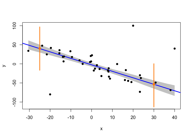
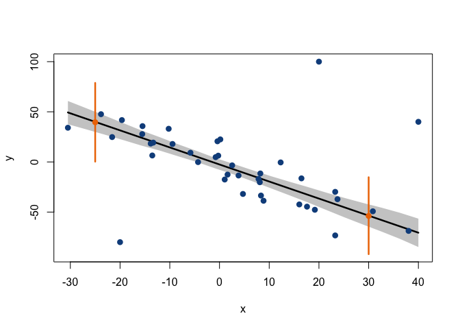
In the plot above, the grey area is defined by the 95% HPD intervals of the regression line (given by the posterior distributions of alpha and beta) at each of the x-values in x_cred. These HPD intervals correspond to the shortest intervals that capture 95% of the posterior probability of the position of the regression line (with this posterior probability being analogous to that shown in the illustration at the beginning of this post, but with the heavier tails of a t-distribution). A very interesting detail is that, while the confidence intervals that are typically calculated in a conventional linear model are derived using a formula (which assumes the data to be normally distributed around the regression line), in the Bayesian approach we actually infer the parameters of the line’s distribution, and then draw random samples from this distribution in order to construct an empirical posterior probability interval. Thus, these HPD intervals can be seen as a more realistic, data-driven measure of the uncertainty concerning the position of the regression line.
The same applies to the prediction intervals: while they are typically obtained through a formulation derived from a normality assumption, here, MCMC sampling is used to obtain empirical distributions of response values drawn from the model’s posterior. In each MCMC sampling iteration, a value for the mean response, mu_pred, is drawn (sampled) from the distributions of alpha and beta, after which a response value, y_pred, is drawn from a t-distribution that has the sampled value of mu_pred as its location (see the model code above). Therefore, a Bayesian 95% prediction interval (which is just an HPD interval of the inferred distribution of y_pred) does not just mean that we are ‘confident’ that a given value of x should be paired to a value of y within that interval 95% of the time; it actually means that we have sampled random response values relating to that x-value through MCMC, and we have observed 95% of such values to be in that interval.
To wrap up this pontification on Bayesian regression, I’ve written an R function which can be found in the file rob.regression.mcmc.R, and combines MCMC sampling on the model described above with some nicer plotting and reporting of the results. With this function, the analysis above becomes as easy as the following:
source("rob.regression.mcmc.R")
reg.noisy3 = rob.regression.mcmc(x=points.noisy$x, y=points.noisy$y,
                                 x.pred=x.pred,
                                 pred.int=90, cred.int=95,
                                 iter=2000, warmup=500, chains=4, seed=911,
                                 xlab="x", ylab="y")
##
## SAMPLING FOR MODEL 'robust_regression' NOW (CHAIN 1).
##
## Gradient evaluation took 1.7e-05 seconds
## 1000 transitions using 10 leapfrog steps per transition would take 0.17 seconds.
## Adjust your expectations accordingly!
##
##
## Iteration:    1 / 2000 [  0%]  (Warmup)
## Iteration:  200 / 2000 [ 10%]  (Warmup)
## Iteration:  400 / 2000 [ 20%]  (Warmup)
## Iteration:  501 / 2000 [ 25%]  (Sampling)
## Iteration:  700 / 2000 [ 35%]  (Sampling)
## Iteration:  900 / 2000 [ 45%]  (Sampling)
## Iteration: 1100 / 2000 [ 55%]  (Sampling)
## Iteration: 1300 / 2000 [ 65%]  (Sampling)
## Iteration: 1500 / 2000 [ 75%]  (Sampling)
## Iteration: 1700 / 2000 [ 85%]  (Sampling)
## Iteration: 1900 / 2000 [ 95%]  (Sampling)
## Iteration: 2000 / 2000 [100%]  (Sampling)
##
##  Elapsed Time: 0.051652 seconds (Warm-up)
##                0.089271 seconds (Sampling)
##                0.140923 seconds (Total)
##
##
## SAMPLING FOR MODEL 'robust_regression' NOW (CHAIN 2).
##
## Gradient evaluation took 1.4e-05 seconds
## 1000 transitions using 10 leapfrog steps per transition would take 0.14 seconds.
## Adjust your expectations accordingly!
##
##
## Iteration:    1 / 2000 [  0%]  (Warmup)
## Iteration:  200 / 2000 [ 10%]  (Warmup)
## Iteration:  400 / 2000 [ 20%]  (Warmup)
## Iteration:  501 / 2000 [ 25%]  (Sampling)
## Iteration:  700 / 2000 [ 35%]  (Sampling)
## Iteration:  900 / 2000 [ 45%]  (Sampling)
## Iteration: 1100 / 2000 [ 55%]  (Sampling)
## Iteration: 1300 / 2000 [ 65%]  (Sampling)
## Iteration: 1500 / 2000 [ 75%]  (Sampling)
## Iteration: 1700 / 2000 [ 85%]  (Sampling)
## Iteration: 1900 / 2000 [ 95%]  (Sampling)
## Iteration: 2000 / 2000 [100%]  (Sampling)
##
##  Elapsed Time: 0.047364 seconds (Warm-up)
##                0.090606 seconds (Sampling)
##                0.13797 seconds (Total)
##
##
## SAMPLING FOR MODEL 'robust_regression' NOW (CHAIN 3).
##
## Gradient evaluation took 1.5e-05 seconds
## 1000 transitions using 10 leapfrog steps per transition would take 0.15 seconds.
## Adjust your expectations accordingly!
##
##
## Iteration:    1 / 2000 [  0%]  (Warmup)
## Iteration:  200 / 2000 [ 10%]  (Warmup)
## Iteration:  400 / 2000 [ 20%]  (Warmup)
## Iteration:  501 / 2000 [ 25%]  (Sampling)
## Iteration:  700 / 2000 [ 35%]  (Sampling)
## Iteration:  900 / 2000 [ 45%]  (Sampling)
## Iteration: 1100 / 2000 [ 55%]  (Sampling)
## Iteration: 1300 / 2000 [ 65%]  (Sampling)
## Iteration: 1500 / 2000 [ 75%]  (Sampling)
## Iteration: 1700 / 2000 [ 85%]  (Sampling)
## Iteration: 1900 / 2000 [ 95%]  (Sampling)
## Iteration: 2000 / 2000 [100%]  (Sampling)
##
##  Elapsed Time: 0.051415 seconds (Warm-up)
##                0.101799 seconds (Sampling)
##                0.153214 seconds (Total)
##
##
## SAMPLING FOR MODEL 'robust_regression' NOW (CHAIN 4).
##
## Gradient evaluation took 1.7e-05 seconds
## 1000 transitions using 10 leapfrog steps per transition would take 0.17 seconds.
## Adjust your expectations accordingly!
##
##
## Iteration:    1 / 2000 [  0%]  (Warmup)
## Iteration:  200 / 2000 [ 10%]  (Warmup)
## Iteration:  400 / 2000 [ 20%]  (Warmup)
## Iteration:  501 / 2000 [ 25%]  (Sampling)
## Iteration:  700 / 2000 [ 35%]  (Sampling)
## Iteration:  900 / 2000 [ 45%]  (Sampling)
## Iteration: 1100 / 2000 [ 55%]  (Sampling)
## Iteration: 1300 / 2000 [ 65%]  (Sampling)
## Iteration: 1500 / 2000 [ 75%]  (Sampling)
## Iteration: 1700 / 2000 [ 85%]  (Sampling)
## Iteration: 1900 / 2000 [ 95%]  (Sampling)
## Iteration: 2000 / 2000 [100%]  (Sampling)
##
##  Elapsed Time: 0.049501 seconds (Warm-up)
##                0.090923 seconds (Sampling)
##                0.140424 seconds (Total)
## SIMPLE LINEAR REGRESSION: POSTERIOR STATISTICS
## Intercept (alpha)
##    Posterior mean and standard deviation: Mean = -2.511587, SD = 2.633975
##    Posterior median and MAD:              Median = -2.499511, MAD = 2.601219
##    Values with 95% posterior probability: 95% HPDI = [-7.968016, 2.377242]
##    Values with 99% posterior probability: 99% HPDI = [-9.411131, 4.311721]
##
## Slope (beta)
##    Posterior mean and standard deviation: Mean = -1.703649, SD = 0.1693493
##    Posterior median and MAD:              Median = -1.701762, MAD = 0.1616968
##    Values with 95% posterior probability: 95% HPDI = [-2.050323, -1.382492]
##    Values with 99% posterior probability: 99% HPDI = [-2.146778, -1.241661]
##
## Predicted value #1 (x = -25)
##    Posterior median predicted response:   Median = 39.59248
##    Values with 90% posterior probability: 90% HPDI = [0.2932198, 78.80611]
##    Values with 95% posterior probability: 95% HPDI = [-20.41053, 94.86489]
##    Values with 99% posterior probability: 99% HPDI = [-118.8511, 174.5186]
##
## Predicted value #2 (x = 30)
##    Posterior median predicted response:   Median = -53.84294
##    Values with 90% posterior probability: 90% HPDI = [-91.99497, -15.24352]
##    Values with 95% posterior probability: 95% HPDI = [-106.2877, 3.749163]
##    Values with 99% posterior probability: 99% HPDI = [-169.6304, 123.0802]
The function returns the same object returned by the rstan::stan function, from which all kinds of posterior statistics can be obtained using the rstan and coda packages. As can be seen, the function also plots the inferred linear regression and reports some handy posterior statistics on the parameters alpha (intercept), beta (slope) and y_pred (predicted values).
All the arguments in the function call used above, except the first three (x, y and x.pred), have the same default values, so they don’t need to be specified unless different values are desired. If no prediction of response values is needed, the x.pred argument can simply be omitted. The arguments cred.int and pred.int indicate the posterior probability of the intervals to be plotted (by default, 95% for ‘credible’ (HPD) intervals around the line, and 90% por prediction intervals). The arguments iter, warmup, chains and seed are passed to the stan function and can be used to customise the sampling. Finally, xlab and ylab are passed to the plot function, and can be used to specify the axis labels for the plot.
Now, what’s your excuse for sticking with conventional linear regression?