While working with a rather large set of human germline polymorphisms, I recently asked myself whether the age of a given variant allele (or mutation) could be estimated from its allele frequency (the fraction of alleles at the relevant locus that are represented by the variant allele). Unsurprisingly, the answer seems to be ‘yes’ up to a certain degree — that is, provided that one is willing to settle for an ideal (and somewhat boring) population, to neglect some of the most important forces that shape population dynamics in the real world, and to accept a great deal of uncertainty in the answer. Nevertheless, looking at what is left after all these concessions are made — that is, the background force behind the most elementary patterns of mutation spread — is quite a nice exercise in itself, and provides a beautiful glimpse of a multidimensional probability distribution.

Thus, my aim here is to examine the probability distribution of the time (number of generations) that a mutation takes to successfully spread (or diffuse) through a population, as a function of the population size (number of individuals) and of the arbitrary threshold allele frequency that constitutes the measure of ‘success’.

At the point where a mutation appears de novo in a population of N individuals, it is naturally found in just one allele; and so the initial allele frequency, f₀, is equal to 1/N for a haploid population, or 1/(2N) for a diploid population. For haploid, asexually reproducing organisms, the evolution of this allele frequency over time is largely deterministic, and can be predicted provided that we know the relative increase or decrease in the rate of replication (or survival) conferred by the mutation. (If the mutation does not affect the replication rate of carriers compared to non-carriers, then its frequency should stay constant, at least in an experimental setting.) If we denote this relative rate difference by w, then, by definition, the frequency ratio between the mutant and wild-type alleles at generation g+1 is given by

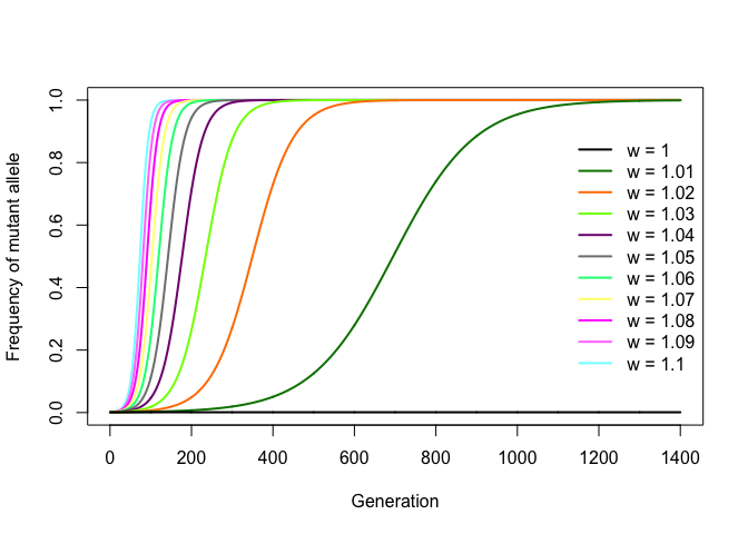
An interesting consequence of this is that one can infer the value of w by fitting this expression to a set of experimentally obtained allele frequencies per generation. If, for example, w = 1.05, then the mutation increases the replication rate by 5% per generation relative to the wild-type allele. Starting from f₀ = 1/N, any value of w > 1 will cause a mutation to gradually spread through the population following a nice sigmoid curve and become fixed (that is, it reaches frequency f = 1), with higher values of w leading to faster fixation. Negative values of w lead to the eventual disappearance (or loss) of the mutation from the population (which ensues immediately if f₀ = 1/N). Thus, w can be seen as a simple proxy for the level of selection for the mutant allele.

The R code below simulates mutation diffusion in a bacterial population for increasing values of w, with f₀ = 1/N.

N = 1000                   # Population size
f0 = 1 / N                 # Initial allele frequency
Ws = seq(1, 1.1, by=0.01)  # Relative mutant replication rates
G = 1400                   # Number of generations

# Simulate for G generations
Fs = sapply(Ws, function(w) {
    f = integer(G)
    f[1] = f0
    for (n in 1:(G-1))
        f[n+1] = (w * f[n]) / (1 - f[n] * (1 - w))
    f
})

# Plot (needs colorRamps package)
cols = colorRamps::primary.colors(ncol(Fs))
plot(Fs[,1], type="n", ylim=c(0, 1), 
     ylab="Frequency of mutant allele", xlab="Generation")
for (j in ncol(Fs):1) {
    lines(Fs[,j], col=cols[j], lwd=2)
}
legend("right", lwd=2, col=cols, legend=paste("w =", Ws), bty="n")

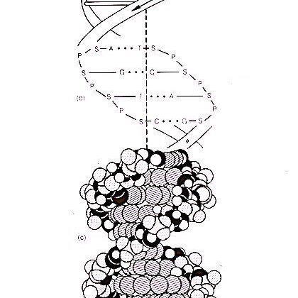
However elegant, this model would be a terrible approximation of a human population, because of complications arising from humans’ propensity to sex. Sexual reproduction involves genetic recombination, which yields non-deterministic offspring genotypes. If, in a diploid species, only one of the parents carries the relevant mutation in one copy of their genome, Mendelian genetics tells us that the probability that the mutation is passed to the offspring is 1/2. In addition, the frequency of an allele in a particular generation is not exactly determined by the frequency in the previous generation, as the genotypes of the offspring will depend on the particular mating between parents, which most models assume to be random (that is, the alleles in the offspring are randomly sampled from the pool of parental alleles). This makes it possible for allele frequencies to fluctuate in a random fashion, even to the extent of fixation or loss, in the absence of selection, a phenomenon known as genetic drift.

As my interest was in estimating the diffusion time of mutations in the absence of selection, genetic drift models seemed like a good starting point (better than modelling people as bacteria, in any case). If we focus on a given allele present in c_g copies in the current generation (with c_g = f_g ∙ 2N), the number of copies of that same allele in the following generation, c_g+1, follows a binomial distribution parameterised by the total number of alleles in the population in the next generation and the allele frequency in the present generation (which, for a diploid population of assumed constant size, have values 2N and f_g = c_g/(2N), respectively). In other words,

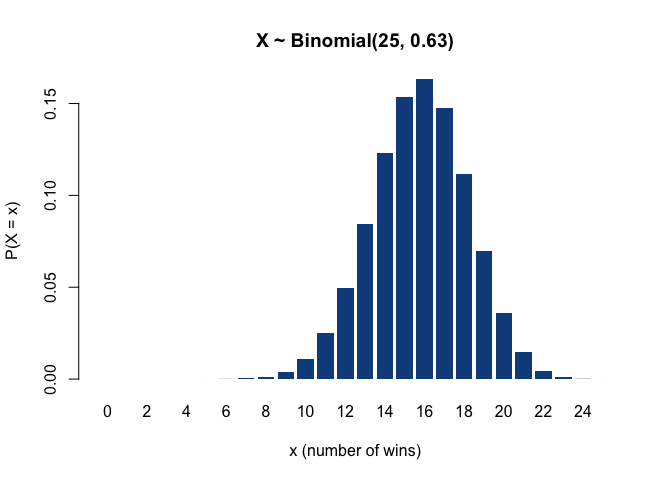
More generally, the binomial distribution models the probability of the number of ‘successes’ after a set of ‘trials’, where the outcome of each individual trial is either success or failure (that is, the outcome of each trial is a binary variable following a Bernoulli distribution). Thus, the binomial distribution describes the sum of multiple Bernoulli-distributed variables. For example, if the New York Yankees have 25 games left to play this season, and their winning rate, i.e. the current proportion of victories to the number of games played so far, is 0.63, then the probability that they will win the next game is 63% (that is, the next game’s outcome is Bernoulli-distributed with success probability 0.63), and the number of victories out of the 10 remaining games, which corresponds to the sum of 10 such Bernoulli variables, is binomially distributed as 𝓑(n = 25, p = 0.63), having an expected value of 25 ∙ 0.63 = 15.75 wins.

(Incidentally, as far as I could find out, the values n = 25 and p = 0.63 are the Yankees’ actual number of remaining games and winning rate for this season – but I wouldn’t recommend making any bets based on the plot below.)

barplot(dbinom(x=0:25, size=25, prob=0.63),
        col="dodgerblue4", border=NA, names.arg=0:25, 
        xlab="x (number of wins)", ylab="P(X = x)", main="X ~ Binomial(25, 0.63)")

Moving permanently away from baseball and back to genetics, the probability of having k copies of a given allele (let’s name it A) in the offspring, given that there are i copies of the allele in the parents and that mating is random, can be seen as the outcome of a process where 2N child alleles (each one representing a ‘trial’) are randomly sampled from the pool of 2N parental alleles. As the sampling is completely random, the probability of any sampled allele being allele A (i.e. the ‘success’ probability) is equal to the frequency of said allele in the parental pool: f = i/(2N). The binomial distribution defines the probability of each value of the number of successes, k (0 ≤ k ≤ 2N), as the product of the probability of obtaining a combination of 2N alleles featuring k copies of A, and the total number of possible such combinations that can be obtained from the pool of 2N parental alleles.

Of course, the frequency of allele A in the present generation, f_g = i/(2N), will likewise follow a binomial distribution that depends on the allele frequency in the previous generation, f_g–1, which in turn depends on f_g–2, and so forth. So the distribution for the number of alleles in any given generation incorporates all these ‘nested’ binomials from each previous generation, like a set of matryoshka dols. Therefore, one would expect the spread of the distribution (that is, the uncertainty) to increase over generations, so that at some point there is a good chance of having many copies of A, but also a good chance of having no copies at all.

Before continuing, it is necessary to explain the limitation of such a mutation model. In the first place, we are assuming random mating among the N individuals that compose the population, so that the alleles in each individual are equally likely to be passed on to the next generation. This means that N is not the actual size of the population (the census population size), but instead it is the effective population size, as it considers only individuals that produce offspring. Second, the model ignores several factors which contribute to the evolution of population allele frequencies over time, most notably selection (which itself operates differently on dominant and recessive alleles), population size changes, migration flows and historical population dynamics (including population bottlenecks). Consequently, what the model represents is but the behaviour of alleles diffusing through an ideal, still population that is unaffected by any of these very natural processes; and, as such, its ability to faithfully represent the dynamics of mutation diffusion in real populations — particularly human populations — is very limited. All this said, the probabilistic patterns that emerge from the mere cumulative action of undisturbed genetic drift are fascinating in their own right, and reveal the background canvas upon which the processes mentioned above often cast their own signatures.

Already in the early days of population genetics, Motoo Kimura and Tomoko Ohta (1969) had employed the diffusion models pioneered by Kimura to analytically determine the average number of generations needed for fixation of a mutation. As Kimura and Ohta mention in their paper,

Since the gene substitution in a population plays a key role in the evolution of the species, it may be of particular interest to know the mean time for a rare mutant gene to become fixed in a finite population, excluding the cases in which such a gene is lost from the population.

The question attracting my interest was slightly different from this: firstly, I was looking for a more general case where a new mutation spreads up to an arbitrary target frequency f < 1, whereas Kimura and Ohta considered only the case where mutations reach f = 1; secondly, I was interested in estimating the probability distribution of the diffusion time — not just the average time — and how the shape of such distribution evolves with changes in population size and target allele frequency.

In any case, I certainly don’t possess anything comparable to Kimura’s mathematical finesse; and although the parameters of the probability distribution of allele copies in generation g can most likely be determined by linking g binomial distributions in the right manner — similar to convoluting multiple Bernoulli distributions, or constructing conditional binomials — I haven’t come across the method for convoluting a series of binomial distributions in such a way that each one determines the success probability of the next.

Nevertheless, sometimes that which is complicated to solve analytically can be easily approximated using random simulations; this is precisely the inspiration behind the origin of Monte Carlo methods. As the inventor of modern Markov-chain Monte Carlo, Stanislaw Ulam, amusingly recalls:

The first thoughts and attempts I made to practice [the Monte Carlo Method] were suggested by a question which occurred to me in 1946 as I was convalescing from an illness and playing solitaires. The question was what are the chances that a Canfield solitaire laid out with 52 cards will come out successfully? After spending a lot of time trying to estimate them by pure combinatorial calculations, I wondered whether a more practical method than “abstract thinking” might not be to lay it out say one hundred times and simply observe and count the number of successful plays.

Just like with Ulam’s solitaire (and more-relevant nuclear physics questions which he addressed), instead of trying to derive the distribution of the number of copies of allele A after g generations (which I suspect may not be that hard to do), we can simulate, say, a thousand de novo mutations in a thousand different populations and observe how they diffuse. So, given a target allele frequency f_t, all we need to do is to introduce each mutation with an initial frequency f₀ = 1/(2N), and wait until the mutation either is lost from the population (in which case we repeat the simulation) or reaches the target frequency f_t, purely by the effect of random drift. Although this simulation experiment is quite easy to set up, we will see how the statistical trends of population genetics build up and progressive hinder the simulation’s progress.

The structure of the simulation will be as follows: we first define a series of target allele frequencies, F_t, a series of (effective) population sizes, N, and a fixed number of repetitions (successful mutations) per simulation setting, M, where each setting involves a specific combination of f_t ∈ F_t and N ∈ N.

Therefore, for each combination of values f_t ∈ F_t and N ∈ N selected from the sets above, we will simulate independent mutations with f₀ = 1/(2N), follow their progression until M of them have reached f_g = f_t, and look at the distribution of the number of generations elapsed, g. We will also count the number of mutations that were lost (that is, reached f_g = 0) during the course of each simulation, and count the number of generations until each loss. As we are only looking at M = 1000 successful mutation diffusions, it makes sense to count the number of generations until loss for the first M lost mutation only; after this, we keep counting subsequent losses, but we no longer count the number of generations elapsed before each, as 1000 samples should be enough to infer the distribution of g.

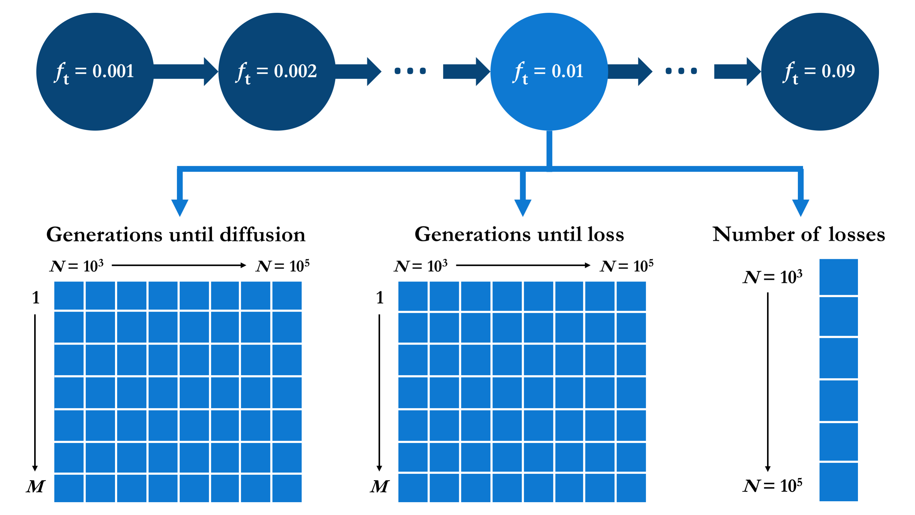
There are different ways in which the values resulting of the series of simulations described could be structured. I opted for organising the output using the target allele frequency as the first grouping level, such that the output for each value of f_t is grouped into the same element of a list. For each f_t, the corresponding element of this list is itself a list containing the three types of relevant output: two matrices of dimensions M × |N| containing the numbers of generations elapsed before the first M successful mutation diffusions and the first M mutation losses, respectively, for each N ∈ N; plus a vector of length |N| containing the total number of mutation losses encountered during the simulation (that is, before the M-th successful diffusion), for each N ∈ N. This output data structure is outlined in the diagram below.

In R, this structure is initialised as follows.

Ns = seq(1e3, 1e5, by=1e3)                # 100 values
Fts = as.numeric(outer(1:9, 10^(-3:-2)))  # 18 values
M = 1000

mut.diffusion = structure(vector(mode="list", length=length(Fts)),
                          names=paste0("ft=", Fts))

for (i in seq(Fts)) {
    mut.diffusion[[i]] = 
        list("g.diff" = matrix(NA, nrow=M, ncol=length(Ns),
                               dimnames=list(NULL, paste0("N=", Ns))),
             "g.loss" = matrix(NA, nrow=M, ncol=length(Ns),
                               dimnames=list(NULL, paste0("N=", Ns))),
             "n.loss" = structure(integer(length(Ns)), 
                                  names=paste0("N=", Ns)))
}

The result is a list (mut.diffusion) of |F_t| = 18 elements, each of which is a list containing two matrices (g.diff and g.loss) and a vector (n.loss), appropriately named with the corresponding values of f_t and N.

names(mut.diffusion)

##  [1] "ft=0.001" "ft=0.002" "ft=0.003" "ft=0.004" "ft=0.005" "ft=0.006"
##  [7] "ft=0.007" "ft=0.008" "ft=0.009" "ft=0.01"  "ft=0.02"  "ft=0.03" 
## [13] "ft=0.04"  "ft=0.05"  "ft=0.06"  "ft=0.07"  "ft=0.08"  "ft=0.09"

str(mut.diffusion$`ft=0.001`)

## List of 3
##  $ g.diff: logi [1:1000, 1:100] NA NA NA NA NA NA ...
##   ..- attr(*, "dimnames")=List of 2
##   .. ..$ : NULL
##   .. ..$ : chr [1:100] "N=1000" "N=2000" "N=3000" "N=4000" ...
##  $ g.loss: logi [1:1000, 1:100] NA NA NA NA NA NA ...
##   ..- attr(*, "dimnames")=List of 2
##   .. ..$ : NULL
##   .. ..$ : chr [1:100] "N=1000" "N=2000" "N=3000" "N=4000" ...
##  $ n.loss: Named int [1:100] 0 0 0 0 0 0 0 0 0 0 ...
##   ..- attr(*, "names")= chr [1:100] "N=1000" "N=2000" "N=3000" "N=4000" ...

mut.diffusion$`ft=0.001`$g.diff[1:4, 1:8]

##      N=1000 N=2000 N=3000 N=4000 N=5000 N=6000 N=7000 N=8000
## [1,]     NA     NA     NA     NA     NA     NA     NA     NA
## [2,]     NA     NA     NA     NA     NA     NA     NA     NA
## [3,]     NA     NA     NA     NA     NA     NA     NA     NA
## [4,]     NA     NA     NA     NA     NA     NA     NA     NA

As described above, for each simulation setting (that is, for each choice of f_t and N), the evolution of each mutation’s frequency over time can be simulated by means of repeated random sampling from the binomial distribution, which is trivial to do in R.

# For a given choice of ft and N, simulate M mutations
for (i in 1:M) {
    
    # Introduce mutation: generation = 0, frequency = 1/(2N)
    g = 0
    f = 1 / (2*N)
    
    while (f < ft) {
    
        # Draw number of allele copies in the next generation:
        # c(g+1) ~ Binomial(2N, f(g) = c(g)/(2N))
        c = rbinom(n=1, size=2*N, prob=f)
        
        # Update allele frequency and generation count
        f = c / (2*N)
        g = g + 1
        
        # If the mutation is lost
        if (c == 0) {
            
            ## (Missing: Update number of losses in `n.loss`
            ## and store number of generations elapsed in `g.loss`)
            
            # Restore initial conditions (reintroduce mutation)
            g = 0
            f = 1 / (2*N)
            
        }
    }
    
    ## (Missing: Store number of generations elapsed in `g.diff`)
}

For simplicity, the code above is missing the lines where results are recorded in the mut.diffusion object, as its aim is simply to demonstrate how sampling and updating of the allele frequency is performed, and how mutation loss is handled. The complete code, including the pieces seen above together plus output storage and plotting, can be found in the file mutation_diffusion.R.

It is important to note that, although I chose R out of convenience in this toy experiment, any serious simulation would benefit from the choice of a more efficient language and implementation. Moreover, as the simulations are independent from each other, this problem is extremely amenable to parallel computing.

It is evident that the time consumed by the simulations increases with the product of f_t and N: a fold increase in either the population size or the target frequency entails the same fold increase in the number of alleles corresponding to a given target frequency. Thus, on the lower end of the parameter space defined by our Fts and Ns above (f_t = 0.001, N = 1000), we only need mutations to reach f_t ∙ 2N = 0.001 ∙ 2000 = 2 alleles, while on the higher end we require 0.09 ∙ 2 ∙ 100,000 = 18,000 alleles. This means that the run time will steadily increase as the simulation progresses. However, the real slow-down comes from the behaviour of the mutations themselves. As already described by Kimura and Ohta (1969), we will see that a huge fraction of all newly arising mutations are rapidly lost from the population due to chance:

[A] single mutant gene which appeared in a human population will be lost from the population on the average in about 1.6 log_e2N generations. If N = 10⁴,this amounts to about 16 generations. These results show that a great majority (fraction 1 – 1/(2N)) of neutral or nearly neutral mutant genes which appeared in a finite population are lost from the population within a few generations, while the remaining minority (fraction 1/(2N)) spread over the entire population (i.e. reach fixation) taking a very large number of generations.

Since our simulations won’t finish until M = 1000 successful mutation diffusions are recorded, they will be forced to witness many, many unsuccessful mutations in the meantime. As the fraction of mutation losses increases with N, this contributes to an even greater inflation of the time consumed by the simulations as N and f_t increase. For instance, for N = 100,000, only around one in every 200,000 simulated mutations will be successful!

Indeed, if you run the code in mutation_diffusion.R, you will very soon notice an exponential increase in the run time per 1000 simulations as the parameter values increase. I decided to stop after some 30 hours of allele crunching, having reached only f_t = 0.05; by then the run time was so inflated that it would have taken perhaps two more days to reach f_t = 0.09. As I said before, this problem can be mitigated by writing a proper parallel implementation in a faster language, but that is very much out of the scope of this post.

In relation to Kimura and Ohta’s conclusions, the first thing that we can do with the results in mut.diffusion is to see whether a similar proportion of successful mutations holds for our simulated mutations.

# (The code below uses the colorRamps package)
Ns = seq(1e3, 1e5, by=1e3)
cols = colorRamps::primary.colors(length(mut.diffusion))

plot(NA, type="n", 
     xlim=c(min(Ns), max(Ns)), ylim=c(0, 0.15), las=1, 
     xlab="Effective population size (N)", ylab="Fraction of successful diffusions")

# Plot fraction of lost mutations against N for each ft
for (i in seq(mut.diffusion)) {
    losses = mut.diffusion[[i]]$n.loss
    lines(x=Ns, 
          y=(1000 / (1000 + losses)), 
          col=cols[i], lwd=1.5)
}

# Add Kimura and Ohta's prediction
points(x=Ns,
       y=(1 / (2 * Ns)),
       pch=16, cex=0.7)

legend("right", legend=names(mut.diffusion), 
       lwd=1.5, col=cols, bty="n", cex=0.9)
legend("topright", legend="1 / (2N)", 
       pch=16, bty="n", cex=0.9, inset=c(0.01, 0))

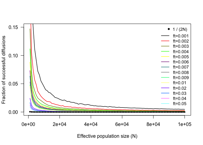
The fraction of successful mutations rapidly converge towards Kimura and Ohta’s 1/(2N) prediction (indicated by the black dots), which of course refers to the case of allele fixation (f_t = 1). Thus, the difference between the observed and predicted fractions can be interpreted as mutations that, although considered ‘successful’ according to our target allele frequency, would eventually become lost before reaching fixation. Naturally, this difference is larger for smaller values of N and f_t.

Let’s finally take a look at the object of our interest: the probability distribution of time to allele diffusion as a function of N and f_t, which we can approximate using the random samples in g.diff. The histogram below shows the distribution of the mutation diffusion time for f_t = 0.01 and three different choices of N.

par(mfrow=c(3, 1), mar=c(4, 4, 1.5, 1))
index = c(1, 10, 100)
powers = 3:5

for (i in seq(index)) {
    hist(mut.diffusion$`ft=0.01`$g.diff[, index[i]],
         breaks=100, freq=F, col="dodgerblue4", border=NA,
         xlab=ifelse(i == length(index), "Generations", ""),
         main=bquote(italic("f")["t"] ~ "=" ~ 0.01 * "," 
                              ~ italic("N") ~ "=" ~ 10 ^ .(powers[i])))
}

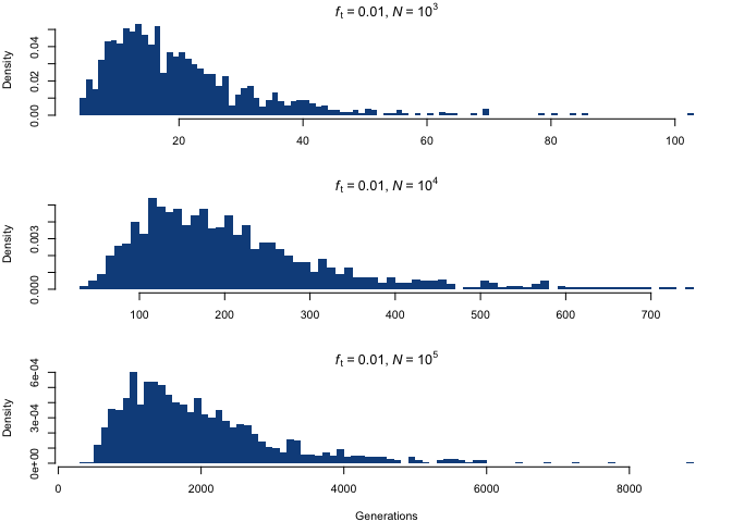
Although the distributions appear to be similar at first, the difference lies in the scaling of the x-axis; by fixing the scale, we see something quite different.

par(mfrow=c(3, 1), mar=c(4, 4, 1.5, 1))
index = c(1, 10, 100)
powers = 3:5

for (i in seq(index)) {
    hist(mut.diffusion$`ft=0.01`$g.diff[, index[i]],
         breaks=100, freq=F, col="dodgerblue4", border=NA,
         xlab=ifelse(i == length(index), "Generations", ""),
         main=bquote(italic("f")["t"] ~ "=" ~ 0.01 * "," 
                              ~ italic("N") ~ "=" ~ 10 ^ .(powers[i])),
         xlim=c(0, 9000))
}

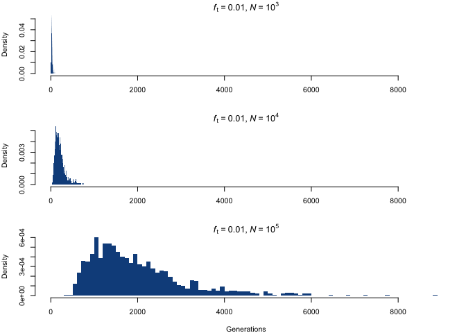
The distribution shifts towards higher values, and acquires much larger spreads, with increasing population size. This scaling up is closely proportional to the increase in N, which is a nice example of the aforementioned property that, for a fixed f_t, a fold increase in N entails the same fold increase in the required number of allele copies.

Although this distribution somewhat resembles a negative binomial, it’s unlikely that it corresponds exactly to any conventional probability distribution, given what it’s meant to represent: it is the distribution of times (generations) that we need to concatenate linked binomial distributions (such that c_g ~ 𝓑(2N, c_g–1/(2N)), c_g–1 ~ 𝓑(2N, c_g–2/(2N)), etc.) before obtaining c_g/(2N) = f_t. However, if this does indeed belong to one of the common distribution families, it would be really great to know which one.

Let’s now look at all values of N at once for f_t = 0.01, by incorporating N to the plots as a second dimension — yes, that means 3D plots!

# Function to plot 3D density
# (uses packages plot3D and colorspace)
plot3d = function(x, y, main) {
    nlevels = 100
    z = table(cut(x, length(unique(x))), cut(y, nlevels))
    z = z / sum(z)
    
    plot3D::persp3D(x=seq(min(x), max(x), len=length(unique(x))),
                    y=seq(min(y), max(y), len=nlevels),
                    z=z,
                    bty="g", expand=0.4, resfac=3, phi=15, theta=110, 
                    inttype=2, border=NA, shade=0.7, nticks=5, ticktype="detailed",
                    col=colorspace::heat_hcl(100), cex.lab=1.2, colkey=list("width"=0.5),
                    xlab="\nEff. population size", ylab="Generations", zlab="Probability")
    title(main=main, cex.main=1.5, line=0)
}

# First, we convert the values in `g.diff` to the 'long format'
Ns = seq(1e3, 1e5, by=1e3)
M = 1000
g.diff.long = cbind("N"=rep(Ns, each=M),
                    "generations"=as.numeric(mut.diffusion$`ft=0.01`$g.diff))
head(g.diff.long)

##         N generations
## [1,] 1000          31
## [2,] 1000          11
## [3,] 1000          21
## [4,] 1000          28
## [5,] 1000          32
## [6,] 1000          10

# Plot distribution of the diffusion time
plot3d(x=g.diff.long[,1],
       y=g.diff.long[,2],
       main=bquote(italic("f")["t"] ~ "=" ~ 0.01))

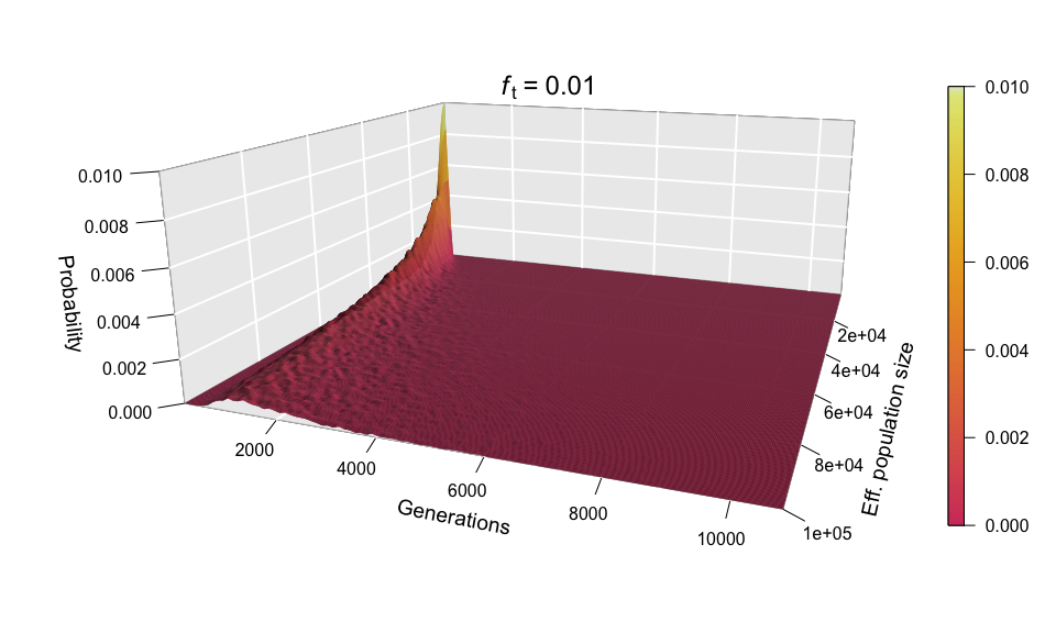
Each of the histograms we saw before was a slice of this two-dimensional probability distribution along the axis labelled ‘Eff. population size’, since each histogram was using a different value of N. Indeed, the slice corresponding to the distribution for N = 100,000 can be seen in the shape of the surface’s cross-section (bottom-left corner of the plot). This plot makes it easier to see how larger population sizes imply larger uncertainty in the diffusion time, while small population sizes curtail the range of possible trajectories that mutations can take before reaching the target frequency, especially for low f_t values (note that f_t = 0.01 corresponds to just 20 allele copies for N = 1000).

Because, as explained above, the values of N and f_t have equal influence on the diffusion time, we shouldn’t be surprised to see that scaling up f_t (for example, to 0.05) produces a scaling of the ‘Generations’ axis analogous to the one seen in the histograms when we increased N.

# Convert the values in `g.diff` to the 'long format'
g.diff.long = cbind("N"=rep(Ns, each=M),
                    "generations"=as.numeric(mut.diffusion$`ft=0.05`$g.diff))

# Plot distribution of the diffusion time
plot3d(x=g.diff.long[,1],
       y=g.diff.long[,2],
       main=bquote(italic("f")["t"] ~ "=" ~ 0.05))

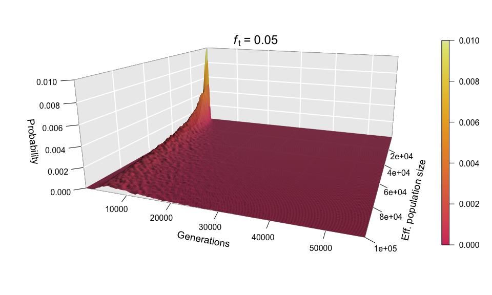
As before, the shape of the distribution hasn’t changed, but the scale has increased (see the ‘Generations’ axis). Just as we did for the histograms, we can fix the scale to see how the distribution expands as f_t increases. We can even go further and consider f_t as an extra dimension of our probability distribution — and as we have already used the three dimensions of space in our 3D plots, the only dimension left is time. In other words, we can sit back and watch the probability distribution of the diffusion time evolve and spread ‘in real time’ as we increase f_t.

This ‘4D’ plot is even better at highlighting the constraint imposed by small values of the population size on the spread of the distribution: while the distribution advances in a wave-like manner for large values of N, there is no room for it to move forward when N is small, as the target frequency is reached very quickly. This gives an interesting pivoting effect, whereby the distribution seems to be ‘sweeping’ the generations axis from a fixed point on the upper left corner. Note that, although the distribution’s spread seems to accelerate over time, this is because the values of f_t > 0.01 that we selected are farther apart than those below 0.01, so the progression seems to become faster after this point. (Note that the target allele frequency is denoted by AF_t in the plot above.)

Another very noticeable thing is the strange backward jump that seems to occur at f_t = 0.09. This appears because the distribution for f_t = 0.08 has a larger spread than it should, based on the pattern followed by all other values, and so the distribution seems to ‘fall back’ to its proper spread at f_t = 0.09. There is, however, no obvious reason why this should happen, as all simulations were conducted in the same way and the spread of the distribution follows quite a deterministic pattern overall.

After seeing the aspect of successful diffusions, let’s take a look at those mutations that didn’t survive. As you will remember, Kimura and Ohta estimated that the great majority of mutations (fraction 1 – 1/(2N)) are lost from the population in about 1.6 log(2N) generations; this corresponds to ~12 generations for N = 1000, and just ~20 generations for N = 100,000. Therefore, we expect practically all the lost mutations to follow a very narrow distribution — and we are not to be disappointed.

# Convert the values in `g.loss` to the 'long format'
g.loss.long = cbind("N"=rep(Ns, each=M),
                    "generations"=as.numeric(mut.diffusion$`ft=0.05`$g.loss))

# Plot distribution of time to loss
plot3d(x=g.loss.long[,1],
       y=g.loss.long[,2],
       main=bquote("Time until mutation loss (" * italic("f")["t"] ~ "=" ~ 0.05 * ")"))

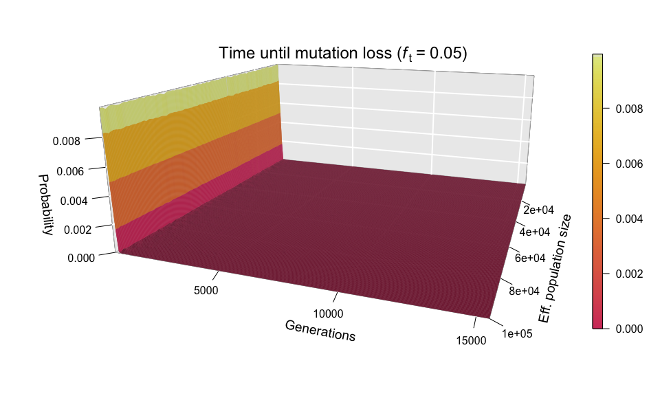
The wall-of-fire plot above confirms Kimura and Ohta’s predictions (at least for a simulated population). Nonetheless, the red carpet along the bottom of the plot provides a very interesting observation: mutations can also be lost by random drift after huge amounts of time. What the red carpet represents are mutations whose allele frequency wandered for a long time (sometimes over 15,000 generations) between zero and f_t (which in the example above is 0.05), before finally disappearing from the population. It is mainly because of these late-losers that the simulation slows down so precipitously as f_t increases.

So, thanks for reading all the way down! I think it’s about time that I wrap up this lecture on what was meant to be just a fun 100-line experiment. However, I would really appreciate any suggestions on how to expand this naive model in interesting ways or further explore its output. I would also be very interested in learning how the convolution of binomials described here can be done analytically, and what, if any, might be the family of probability distributions that describes the diffusion time for a given choice of f_t and N.