Sampling in the hypersphere
Adrian Baez-Ortega
14 October 2018
This post is the first of a short series where I will be presenting some of the most remarkable concepts and techniques from the field of statistical physics, all of which are beautifully featured in Werner Krauth’s marvelous book Statistical Mechanics: Algorithms and Computations (Oxford University Press). (As a side note, I positively recommend Krauth’s related free online course, which is every bit as delightful as his book, and more accessible to those lacking a physics background.)
The problem in focus today is deceptively simple: how to efficiently sample random points inside a sphere. Such sphere, however, may be defined not in the familiar three dimensions, but in any number of dimensions. We shall see that an intuitive but naive sampling strategy, even though at first provides a solution, is notwithstanding bound to become exceptionally inefficient as the number of dimensions, D, increases; and, in our way towards a superior sampling algorithm, we shall encounter some captivatingly clever and powerful mathematical conceptions, including sample transformations and isotropic probability distributions.
Let us begin by defining the objects in question. We use the term hypersphere to refer to the general version of the sphere in an arbitrary number of dimensions. Thus, the two-dimensional hypersphere and the three-dimensional hypersphere correspond, respectively, to what we normally call a circle and a sphere. Hyperspheres with many more dimensions can also be defined, even if our capacity for picturing them is impaired by our everyday experience of three-dimensional space (try for a moment to imagine the aspect of a sphere in four dimensions!). In order to save ourselves from having to read many long words, however, we shall refer to hyperspheres simply as spheres. In addition, we only consider, for simplicity, the case of the unit sphere, which has a radius r = 1.
Analogously, the hypercube is the general version of the cube in any dimensions, and we shall simply call it the D-dimensional cube. We should note that, for D = 1, both the one-dimensional sphere and one-dimensional cube correspond to a straight line segment.
The reason why cubes are of interest here, is that they are instrumental in the simplest and most intuitive way of sampling random points inside a sphere. Let us consider, for example, the sphere in two dimensions — that is, the circle. The most obvious technique for sampling points inside a circle is to first sample random points (pairs of x and y coordinates) inside a square containing the circle, and then accepting each random point as valid only if it is indeed inside the circle (that is, if its distance to the centre is smaller than the circle radius).
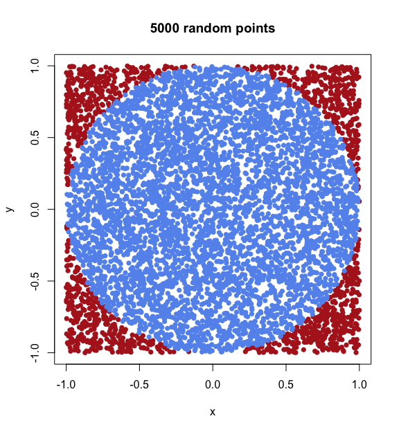
We can easily write a short algorithm for this naive sampling method in R, and plot the resulting points. We will plot any points lying outside the circle (rejected samples) in red, and any points inside the circle (accepted samples) in blue.
# Naive sampling of N random points (each a vector of coordinates
# [x_1, ..., x_D]) inside a D-dimensional sphere of radius r
naive.hypersphere = function(N, D, r=1) {
    set.seed(1)
    samples = list(accepted = matrix(NA, nrow=N, ncol=D),
                   rejected = matrix(NA, nrow=1e6, ncol=D))
    i = j = 0
    while (i < N) {

        # For each dimension (1, 2, ..., D),
        # sample a random coordinate in [-1, 1]
        point = runif(n=D, min=-1, max=1)

        # Check if the point is inside the sphere,
        # i.e., if (x_1^2 + x_2^2 + ... + x_D^2) < r^2
        accept = sum(point ^ 2) < r ^ 2

        # Add to the table of accepted/rejected samples
        if (accept) {
            i = i + 1
            samples$accepted[i, ] = point
        }
        else {
            j = j + 1
            samples$rejected[j, ] = point
        }

    }
    samples$rejected = samples$rejected[1:j, ]
    samples
}
# Sample 1000 random points inside the circle of radius 1
points.circle = naive.hypersphere(N=5000, D=2)

# Plot accepted points in blue and rejected points in red
plot(points.circle$rejected, pch=16, col="firebrick",
     xlab="x", ylab="y", main="5000 random points")
points(points.circle$accepted, pch=16, col="cornflowerblue")
This method can be applied to the sphere in any number of dimensions, as illustrated below for the cases D = 1, 2, 3.
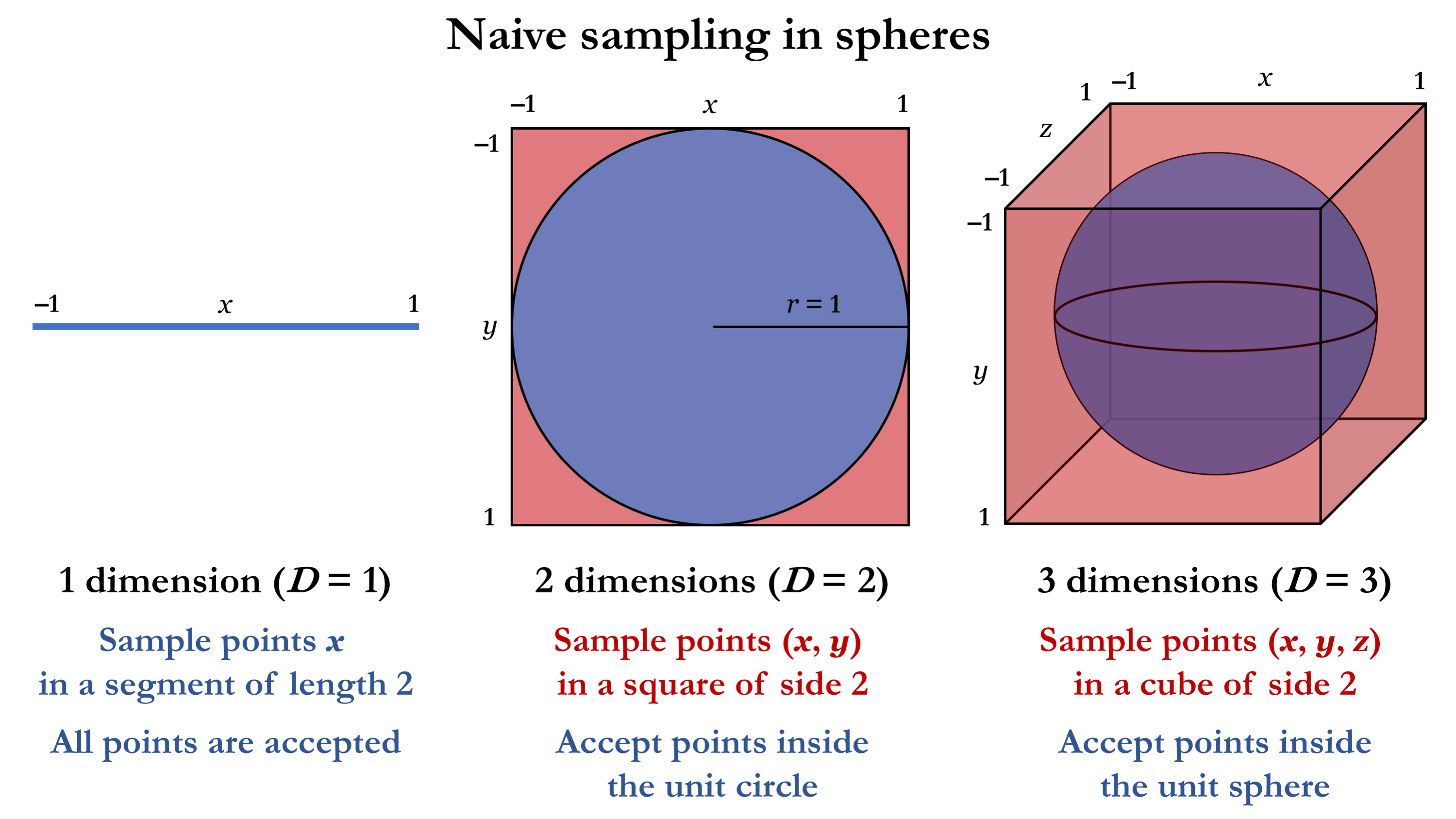
As you might have already noticed, the problem with this sampling algorithm is that the region in which the points are sampled (the cube) and the region where they are accepted (the sphere) rapidly grow more distinct from each other as we go to higher dimensions. While for D = 1 the sampling is perfectly efficient (as both sphere and cube correspond to the same line segment), we already notice that the difference between the 3-dimensional cube and the sphere within is substantially larger than the difference between the 2-dimensional square and its circle. In general, the ratio of the volume of the sphere to that of the cube gives the algorithm’s acceptance rate (the fraction of accepted samples) for D dimensions, as shown below.
| Dimensions | Sphere analogue | Cube analogue | Volume of unit sphere | Volume of cube of side 2 | Acceptance rate |
|---|---|---|---|---|---|
| D = 1 | Line segment | Line segment | VS = length = 2 | VC = length = 2 | VS / VC = 1 |
| D = 2 | Circle | Square | VS = area = 𝜋 | VC = area = 4 | VS / VC = 𝜋 / 4 ≈ 0.79 |
| D = 3 | Sphere | Cube | VS = volume = 4/3 𝜋 | VC = volume = 8 | VS / VC = 𝜋 / 6 ≈ 0.52 |
| ... | ... | ... | ... | ... | ... |
| Large D | Hypersphere | Hypercube | VS = 𝜋 (D / 2) r D / Γ((D / 2) + 1) | VC = 2 D | VS / VC ≪ 1 |
The acceptance rate already drops dramatically for D = 3, foreshadowing the method’s fate in higher dimensions. For large values of D, this method is simply too inefficient to be of any use, as nearly all of the proposed samples are rejected.
As an interesting side note, notice that the number 𝜋 is involved in the acceptance rate; this implies that, as we sample and accept/reject points with this algorithm, we are inadvertently computing the value of 𝜋 to an increasing degree of accuracy. For example, we can approximate 𝜋 from the empirical acceptance rate of our previous sampling exercise on the circle.
# For D = 2:
# Acceptance rate = (accepted samples) / (total samples) = 𝜋 / 4
accept.rate = nrow(points.circle$accepted) /
    (nrow(points.circle$accepted) + nrow(points.circle$rejected))
accept.rate
## [1] 0.7818608
# Approximation of 𝜋
accept.rate * 4
## [1] 3.127443
It seems that we need to sample quite a bit longer before arriving to an acceptable estimate of 𝜋!
We have seen that the acceptance-rate problem derives from the fact that we are sampling from a distribution which does not exactly match the region we are interested in. Let us now turn to a different approach, where the coordinates are sampled not from a uniform distribution between –1 and 1, but from a standard Gaussian (or normal) distribution. We will see that, by applying a clever transformation, a vector of D Gaussian random numbers can be converted into a random point inside the D-dimensional unit hypersphere, or even on its surface. This method achieves rejection-free sampling, meaning that no samples ever fall outside the sphere. Hence, this algorithm will be free from the efficiency concerns of the previous one.
Let us begin by sampling points as vectors of D independent Gaussian coordinates. In two dimensions, we sample two coordinates, x and y, which gives the following distribution of samples.
# Plot 1000 random points in two dimensions,
# each composed of two independent Gaussian random coordinates
plot(x = rnorm(n=1000),
     y = rnorm(n=1000),
     pch=16, col="cornflowerblue", xlab="x", ylab="y", main="1000 random points")
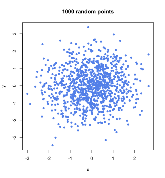
So far, this looks more like a cloud than a circle. The crucial detail here, however, is that the points in this cloud are uniformly distributed in all directions. This is because the combination of two Gaussian distributions gives an isotropic distribution in two dimensions. Isotropic is just a fancy Greek name for something that is uniform in all orientations; in other words, something whose aspect does not change when it is rotated. An orange is normally isotropic, while a banana never is.
The Gaussian distribution has the unique property that the combination of D independent distributions generates an isotropic distribution in D dimensions. This is the key insight that enables rejection-free sampling in a sphere of any dimensionality.
(The proof that the Gaussian distribution is isotropic is itself deeply elegant, but will not be shown here. Briefly, it involves some clever variable transformations on an integral over the Gaussian distribution, resulting in two independent integrals on the angular and radial variables. It then becomes evident that the integral over the angular variable spans all angles uniformly, which is the definition of isotropy.)
Let us now climb from two to three dimensions, where the combination of three independent Gaussian variables (for x, y and z) again produces an isotropic, globular cluster of points.
# Plot 1000 random points in three dimensions (using package plot3D),
# each composed of three independent Gaussian random coordinates
plot3D::points3D(x = rnorm(n=1000),
                 y = rnorm(n=1000),
                 z = rnorm(n=1000),
                 col="cornflowerblue", pch=16, alpha=0.7,
                 bty="g", phi=20, main="1000 random points")
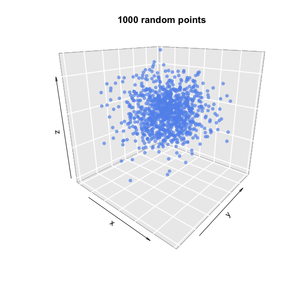
Now, all we have to do is reshaping this cloud into a perfect sphere. This requires transforming the distances, or radii, of the points, so that points are uniformly distributed across all radii. Because the volume increases exponentially with distance from the centre, however, longer radii demand more points than shorter ones (consider how many points would be needed in order to fill the space just beneath the sphere’s surface, in contrast with the amount needed to fill the space just around its centre).
To be precise, achieving uniform sampling in terms of radii requires a probability distribution proportional to the (D – 1)-th power of the radius r (with 0 < r < 1):
Fortunately, sampling from this distribution is easy: we only need to sample from a uniform distribution between 0 and 1, and take the D-th root of every sample; the transformed samples will then follow the exponential distribution shown above.
To assign the radii sampled from the distribution above to the points that we sampled from the isotropic Gaussian distribution, we need to divide the value of each coordinate by the point’s original distance (given by the square root of the sum of its squared coordinates), and then multiply the coordinates again by the new radius. After this correction, the points will uniformly cover not just all angles, but also all distances between 0 and 1.
Below is a function that ties all these ideas together into an algorithm for rejection-free sampling of points in a D-dimensional sphere of radius r.
# Rejection-free sampling of N random points (vectors of coordinates
# [x_1, ..., x_D]) in/on a D-dimensional sphere of radius r
gaussian.hypersphere = function(N, D, r=1, surface=FALSE) {

    # Sample D vectors of N Gaussian coordinates
    set.seed(1)
    samples = sapply(1:D, function(d) {
        rnorm(n=N)
    })

    # Normalise all distances (radii) to 1
    radii = apply(samples, 1, function(s) {
        sqrt(sum(s ^ 2))
    })
    samples = samples / radii

    # Sample N radii with exponential distribution
    # (unless points are to be on the surface)
    if (!surface) {
        new.radii = runif(n=N) ^ (1 / D)
        samples = samples * new.radii
    }

    samples
}
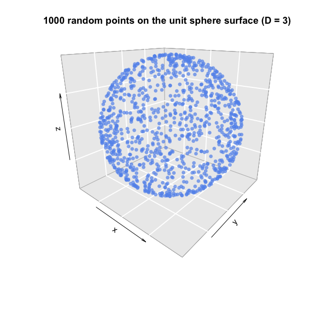
Note that this function includes an additional argument, surface, which allows us to skip the sampling of new radii after the points have been normalised to have radius equal to 1. This results in points which are uniformly distributed on the surface of the sphere, instead of inside it.
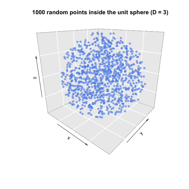
Below are two examples of 1000 random points, inside and on the unit sphere, respectively.
# Sample 1000 random points inside the unit sphere (D=3)
points.sphere = gaussian.hypersphere(N=1000, D=3)
plot3D::points3D(x = points.sphere[, 1],
                 y = points.sphere[, 2],
                 z = points.sphere[, 3],
                 col="cornflowerblue", pch=16, alpha=0.7, bty="g", phi=20,
                 main="1000 random points inside the unit sphere (D = 3)")
# Sample 1000 random points on the surface of the unit sphere (D=3)
points.sphere = gaussian.hypersphere(N=1000, D=3, surface=TRUE)
plot3D::points3D(x = points.sphere[, 1],
                 y = points.sphere[, 2],
                 z = points.sphere[, 3],
                 col="cornflowerblue", pch=16, alpha=0.7, bty="g", phi=20,
                 main="1000 random points on the unit sphere surface (D = 3)")
This rejection-free sampling algorithm, if formally quite simple, provides a powerful example of the importance of understanding the topology of the space in which sampling is to be done, and of the beauty and elegance which so often characterise the mathematical tools, such as variable and sample transformations, that are ubiquitous in statistical physics.
Finally, it must be noted that, although I have chosen to present this sampling approach mainly because of its mathematical ingenuity, hypersphere sampling is not only beautiful, but also of prime importance in statistical mechanics and other branches of physics. To mention one example, the velocities of N classical particles in a gas with constant kinetic energy are distributed as random points on the surface of a 3N-dimensional hypersphere. This is because the fixed kinetic energy is proportional to the sum of the squared velocities, and therefore any valid set of particle velocities (each with x, y and z components) must satisfy that the sum of their squares is proportional to the kinetic energy — just as any point on the surface of a sphere has coordinates whose sum-of-squares is, by definition, equal to the square of the sphere radius.
Interestingly, the distribution of points in a hypersphere is also connected with J. J. Thomson’s landmark 1904 atomic model, which described the atom as a positively charged sphere with negatively charged electrons embedded in it. More generally, the problem of carefully defining the sampling space is of foremost importance in Markov chain Monte Carlo sampling, being the motivation behind some of the most advanced methods in the field, such as Hamiltonian Monte Carlo and Adiabatic Monte Carlo.
This post was largely inspired by the contents of Werner Krauth’s book Statistical Mechanics: Algorithms and Computations (Oxford University Press), and its companion online course.