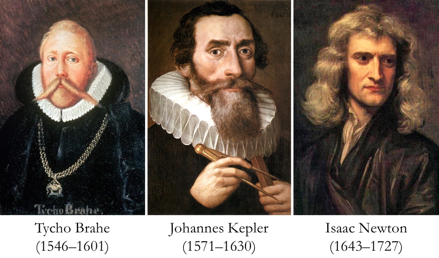
A few days ago I was reading one of the famous Feynman Lectures on Physics, which included a discussion of Kepler’s laws of planetary motion; this is a set of three simple-looking laws proposed by the German astronomer and mathematician Johannes Kepler (1571–1630) to describe the motion of the planets around the Sun.

Kepler, who would eventually become the imperial mathematician to three Holy Roman Emperors, had worked as an assistant to the celebrated Danish astronomer Tycho Brahe (1546–1601). Tycho was a visionary astronomer who had revolutionised the field through his new approach to science; he defended that scientific truth could be reached only by extremely precise measurement, rather than by logical argumentation. In pursue of this view, he established an impressive astronomical observatory in the then-Danish island of Hven; this was probably the first proper research institute in the world. (Another interesting fact: Tycho lost his nose in a sword duel with another nobleman in 1566, after a quarrel over who was the best mathematician(!), and for the rest of his life wore an prosthetic nose made of brass.)

Kepler made use of the extensive and incredibly accurate astronomical tables that Tycho had compiled through decades of work, and arrived at a set of laws describing the motions of the planets around the Sun (although he didn’t publish them in the form of three laws, as they are known today). Subsequently, Isaac Newton (1643–1727) would build on Kepler’s laws to arrive at his own law of universal gravitation. In a beautiful cross-generational chain of knowledge, Newton’s law came to explain the forces responsible for the movements of the planets as they had been observed by Tycho a century before, and then described by Kepler’s laws.

You will probably remember Kepler’s laws of planetary motion from your elementary physics classes. (Just kidding.) The three laws are as follows:

1. The orbit of a planet is an ellipse with the Sun at one of the two foci.
2. A line segment joining a planet and the Sun sweeps out equal areas during equal intervals of time.
3. The square of the orbital period of a planet is directly proportional to the cube of the semi-major axis of its orbit.

The second of these laws, which is perhaps the most famous one, always strikes me for its simplicity. The fact that, as a planet orbits a star, the radius of its orbit sweeps out equal areas in equal times seems just too neat. As Newton would prove, this results from the manner in which the intensity of the gravitational field decreases with the square of the distance, and explains why planets move faster when they are closer to the star. So, as I read Feynman’s description of Kepler’s laws, I realised that it would be possible, and very interesting, to simulate an idealised Solar System entirely from the knowledge contained in these laws — in particular the first two — and a bit of trigonometry.

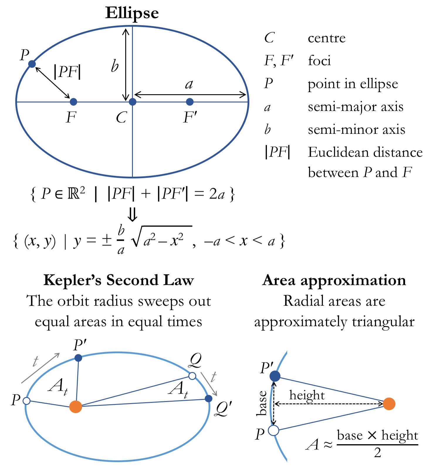
It took surprisingly little time to work out the few tools required for this task. As I wanted to do most of the thinking myself, I avoided an exact formulation for the area of a radial section of an ellipse, and opted instead for a geometric approximation. Concretely, the area of the radial section of the ellipse that is swept by the orbit radius between two positions P and P′ can be approximated by the area of a triangle with vertices P, P′ and F (the ellipse focus, where the star is). If the distance between P and P′ is very small relative to the circumference of the ellipse, then the error introduced by this approximation is negligible. Incidentally, the geometry implied in this approximation gives a nice illustration of the link between the Euclidean distance and the Pythagorean theorem: the Euclidean distance between two points is the length of the hypotenuse of a right triangle whose other two sides are given by the differences between the coordinates of the two points.

Apart from the area formulation described above, the only piece of knowledge required is the formula that describes the y-coordinates of the points along an ellipse as a function of their x-coordinates. This derives from the mathematical definition of an ellipse as the set of all points (x, y) such that the sum of the distances between each of the foci (F and F′) and the point is equal to twice the semi-major axis of the ellipse (usually denoted by a).

The figure below presents the concepts involved in the definition of an ellipse and the approximation of the radial areas referred to in Kepler’s second law.

I will show how to implement this in the R language, while relying as little as possible on R-specific functionalities. For instance, although R already has a function for the Euclidean distance, we will start by implementing this ourselves, together with a function for calculating the area of the triangle defined by two ellipse points (P, Q) and the ellipse focus (F).

# Euclidean distance between two points
distance = function(P, Q) {
    sqrt((P[1] - Q[1]) ^ 2 + (P[2] - Q[2]) ^ 2)
}

# Triangular area between two orbit positions and focus
triangle.area = function(P, Q, F1) {
    base = distance(P, Q)
    height = sqrt(distance(P, F1) ^ 2 - (base / 2) ^ 2)
    base * height / 2
}

Now, we define a set of orbits. For this, it is useful to have a function that calculates the y-value (ordinate) corresponding to a given x-value (abscissa) on the circumference of the ellipse; thereby we can obtain the coordinates of points in the ellipse for a range of values along x. We use the formula relating y and x for the ellipse, shown in the figure above. The formula needs to be modified, however, to account for the fact that the ellipses will have different centres — instead of being all centred at (0, 0). In addition, we need to specify whether we want the y coordinate for the point in the upper half of the ellipse, or the one in the lower half (note the ± sign in the formula above). Therefore, we add the argument Cx and sign to indicate the x-value of the ellipse centre and the side of the ellipse we are interested in, respectively.

# Obtain Y value for given X value in an ellipse with
# semi-major axis a, semi-minor axis b, and centre abscissa Cx
y.ellipse = function(x, a, b, Cx, sign = 1) {
    sign * (b / a) * sqrt(a ^ 2 - (x - Cx) ^ 2)
}

We define five concentrical orbits, all with their foci at the same position F1. We use a ratio between the major and minor axes of 3/4 (although the actual orbits in our Solar System are almost circular), and we increment the semi-major axis, a, by one unit for each new orbit (this defines how far apart the orbits are). Then we obtain a series of points along each orbit using the y.ellipse function defined above.

# Orbit parameters
N = 5                                   # Number of orbits
K = 1                                   # Orbit scale factor
R = 3 / 4                               # Orbit axis ratio
F1 = c(-K / 2, 0)                       # Orbit focus
a = sapply(1:N, function(n) K * n)      # Semi-major axis per orbit
b = sapply(1:N, function(n) R * K * n)  # Semi-minor axis per orbit
Cx = (a - K) / 2                        # Centre abscissa per orbit

# Fixed positions along each orbit
orbit.pos = lapply(1:N, function(i) {
    x = seq(Cx[i] - a[i], Cx[i] + a[i], 
            length.out = 500)
    rbind(c(x, rev(x)),
          sapply(c(x, rev(x)), y.ellipse, a[i], b[i], Cx[i]) *
              rep(c(-1, 1), each = 500))
})

Let’s now define a function for plotting the orbits and see how they look like.

# Plot orbits
plot.orbits = function(orbits, F1, colours, t) {
    par(mar = rep(0, 4), bg = "black")
    xs = sapply(orbits, `[`, 1, TRUE)
    ys = sapply(orbits, `[`, 2, TRUE)
    xlim = c(min(xs), max(xs))
    ylim = c(min(ys), max(ys))
    plot(NA, type="n", axes=FALSE,
         xlab="", ylab="", xlim=xlim, ylim=ylim)
    for (i in 1:length(orbits)) {
        lines(orbits[[i]][1, ], orbits[[i]][2, ], lwd=2, col=colours[i])
    }
    points(F1[1], F1[2], pch=16, cex=3, col="white")
    text(xlim[1], ylim[2] * 0.94, paste("t", t, sep=" = "), 
         col="white", cex=1.2, adj=0)
}

plot.orbits(orbit.pos, F1, t=0,
            colours=c("orchid1", "turquoise1", "gold", "lawngreen", "red"))

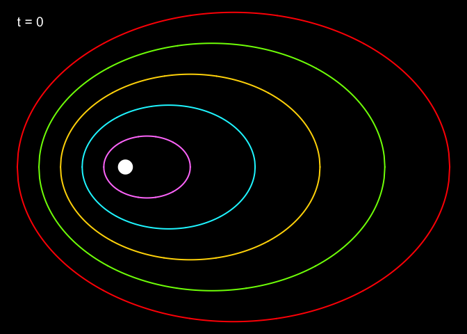
Notice that the white dot, representing the Sun, lies halfway along the negative (left) semi-major axis for each of the ellipses. With this, we have implemented Kepler’s first law: ‘The orbit of a planet is an ellipse with the Sun at one of the two foci’.

Let’s now look at the second law of ‘equal areas in equal times’. If we define a fixed area A_t that each planet must sweep in one time unit, we could apply some non-trivial trigonometry to find the next point along the orbit which results in a triangle with area A_t, and move the planet directly to that point. Instead, I will take an iterative approach, whereby the planet moves forward along its orbit in small steps until it has swept the desired area, and then stops. The step size is obviously critical: if steps are too short, the simulation will be inefficient, whereas if they are too long, the swept area will tend to be excessive. In addition, we need to carry the ‘sign’ of the planet’s movement; that is, whether the planet is moving along the lower half or the upper half of the orbit (as the direction of the movement is the opposite in each half). This ‘sign’ is stored in the same vector that contains the coordinates of the current orbit position, P.

# Move from current orbit position to the closest position
# resulting in a swept area ≥At
next.orbit.pos = function(P, a, b, Cx, delta, F1, At) {
    area = 0
    x = P[1]
    sign = P[3]
    while (area < At) {
        x = x + sign * delta
        if (x < Cx - a) {
            x = Cx - a
        }
        else if (x > Cx + a) {
            x = Cx + a
        }
        y = y.ellipse(x, a, b, Cx, sign)
        if ((y == 0) | (sign < 0 & y > 0) | (sign > 0 & y < 0)) {
            sign = -sign
        }
        area = triangle.area(P, c(x, y), F1)
    }
    c(x, y, sign)
}

With this, we have implemented Kepler’s second law. I have intentionally shunned the third law (which relates the orbital period with the orbit’s semi-major axis) for two reasons. First, adjusting the orbital periods according to this law would require knowing the periods in the first place, which is not straightforward in this setting. Because the motions here arise directly from the second law, and not from equations describing the velocities and accelerations of the planets, we cannot predict their periods, but only discover them as the simulation progresses. (In fact, we could predict the periods by dividing the ellipse into triangles of area A_t and counting the number of triangles, but this would be like running the simulation before running the simulation.)

Second, the third law states that the square of the orbital period is proportional to the cube of the semi-major axis; in other words, planets with larger orbits take much longer to complete them (for instance, Saturn has an orbital period of 29.5 years). However, if we think in terms of the second law, a larger orbit also implies that the movement needed to sweep a fixed area is much smaller (as the radius is longer), so by imposing the second law across all orbits, we are already slowing down the motion of the planets with larger orbits. So it’s not clear to me whether Kepler’s third law could be interpreted as a consequence of the second, or would need to be enforced independently — although I presume the latter.

The only thing left to do is actually running the simulation and plotting the motions of our toy Solar System. For each time-step in the simulation, the code below plots the current orbit positions to a PDF file, and moves each planet to its next position according to Kepler’s second law. The full code is available in the script kepler_orbits.R.

# Simulation parameters
D = 5e-5  # Minimum step size
At = 0.1  # Area swept per time-step
Nt = 1e3  # Number of simulation time-steps

pdf("kepler.pdf", 5, 4)
COL = c("orchid1", "turquoise1", "gold", "lawngreen", "red")

# Initialise orbit positions
positions = rbind(sapply(orbit.pos, `[`, TRUE, 1), sign = 1)

# For each time-step
for (i in 1:Nt) {
    # Plot current orbit positions
    plot.orbits(orbit.pos, F1, COL, i)
    points(positions[1, ], positions[2, ], col=COL, pch=16, cex=2)
    
    # Calculate next position for each orbit
    positions = sapply(1:ncol(positions), function(j) {
        next.orbit.pos(positions[, j], a[j], b[j], Cx[j], D, F1, At)
    })
}

dev.off()

The resulting animation is a quite convincing reproduction of the planetary motions; notice how the planets are ‘slingshot’ away when they come close to the star. Although a mathematical description of the underlying forces would have to wait for Newton, Tycho recorded the motions of the planets so excellently, and Kepler condensed their properties so neatly, that today we are able to reproduce them without any resort to the theory of gravitation. As I thought when reading Feynman’s text, it’s almost unbelievable how much information there is in the words ‘equal areas in equal times’.